Prediction Markets II
Posted: 2018-08-08.
In this follow-up on an introduction to prediction markets, they are back and badder than ever with a more formal and general mathematical approach.
This is the theoretical approach to prediction markets often studied in the computer science and economics literature. It uses a centralized "automated market maker" with which all traders interact, rather than matching them to buy and sell with each other. This setup does not always match what is used in practice, but it's a clean model we can prove things about. The main reference is Abernethy, Chen, and Wortman Vaughan (2013). We'll start by describing cost function based prediction markets, then return to scoring rule based markets and the convex duality connection between them.
Helpful reading for this post includes the above intro to prediction markets as well as scoring rules for eliciting expectations.
Cost Function Based Markets
We will have an observable event $\omega \in \Omega$, which let's say is a finite set because, after all, who among us has ever witnessed the infinite? (The theory does extend.) The goal is to predict a random variable $\phi: \Omega \to \mathbb{R}^d$ (in previous posts this was $Y$). We will find it useful to think of each coordinate as a separate function $\phi_1,\dots,\phi_k$ where $\phi_i : \Omega \to \mathbb{R}$.
High-level idea. Our market will consist of a separate "security" for each coordinate $i=1,\dots,d$. Traders arrive to the market sequentially, one at a time. Each trader $t=1,\dots,T$ can buy or sell "shares" in any of the securities.
The idea is going to be that owning a "share" of security $i$ pays off $\phi_i(\omega)$ when the event $\omega$ is observed. So if the current price of security $i$ is less than $\mathbb{E} \phi_i(\omega)$, then a trader can expect to make money by purchasing a share; vice versa if it's higher. So prices should converge to the expected values of the random variables.
For that to happen, the prices had better go up when people buy shares and down when they sell them. This is achieved by a "cost function" that determines how to set prices based on the history of transactions.
Formalization. Concretely, the designer (also called market maker) initializes a vector $\theta^0 \in \mathbb{R}^d$ by setting $\theta^0 = \vec{0}$. When each participant $t=1,\dots,T$ arrives, she specifies a vector $d\theta^t \in \mathbb{R}^d$, giving the number of shares in each security that she wishes to purchase; and the designer sets $\theta^t = \theta^{t-1} + d\theta^t$. We call $\theta^t$ the market state at time $t$, and it tracks the total number of shares purchased in each security up to and including the $t$th participant.
To set the price of each purchased bundle, the market maker chooses ahead of time a convex cost function $C: \mathbb{R}^d \to \mathbb{R}$, and requires that $C(\theta)$ is the total price paid so far by all participants.
Thus, participant $t$ pays $C(\theta^t) - C(\theta^{t-1})$, and purchases the share vector $d\theta^t = \theta^t - \theta^{t-1}$. Her payoff for these shares, when $\omega$ is observed, is $d\theta^t \cdot \phi(\omega) = \sum_{i=1}^d d\theta^t_i \phi_i(\omega)$.
Interpreting Prices
But wait -- the point of the prediction market was to, uh, well, what are the predictions here exactly?
I said above that the prices can be interpreted as predictions. But the prices are a bit weird in the cost-function setup -- depending on how much you want to buy, the price is $C(\theta + d\theta) - C(\theta)$, which is not the most intuitive object ever to walk down the block.
The idea is that the derivative of $C$ (or in higher dimensions, the gradient) gives the current instantaneous prices. The only complicating factor is that, as you start buying your bundle $d\theta$ at a price $\nabla C(\theta)$, the prices start changing to incorporate the information you bring. But at the instant you arrive, the price per share is $\nabla C(\theta)$.
To see this, imagine we make a very small transaction, for example, we buy $\epsilon$ shares of security $i$ with $\epsilon \to 0$. What price per share do we pay? \[ \frac{C(\theta + (0,\dots,0,\epsilon,0,\dots,0)) - C(\theta)}{\epsilon} \approx \frac{\partial C(\theta)}{\partial i} . \] In other words, the gradient $\nabla C(\theta)$ gives the current market prediction of $\mathbb{E} \phi(\omega)$. (If $C$ is not differentiable at $\theta$, then the same idea applies to any subgradient of $C$ at $\theta$; all are valid predictions.)
An Important Special Case
An "Arrow-Debreu" security is one that pays off $1$ if a certain $\omega$ occurs and $0$ otherwise. Suppose $\Omega = \{1,2,\dots,k\}$ and we have one Arrow-Debreu security for each state $i \in \Omega$. Somebody (call him Likely Larry) has a belief $p \in \Delta_{\Omega}$, a distribution over possible outcomes. What is Larry's expected payoff for a share of security $i$? It is of course $p_i$, since it equals $1$ with probability $p_i$ and zero otherwise. So this is the kind of market discussed in the previous post.
Reminder: Scoring Rules
Now, in this post I've done something I don't usually like to do, which is go for ten minutes straight without mentioning proper scoring rules. Let's fix that now by recalling that $S: \Delta_{\Omega} \times \Omega \to \mathbb{R}$, which takes a prediction $p$ and observed outcome $\omega$, is strictly proper if $\mathbb{E}_{\omega \sim p} S(p,\omega) \gt \mathbb{E}_{\omega \sim p} S(q, \omega)$ for all $q \neq p$. That is, your expected score (under belief $p$) is uniquely maximized by truthfully reporting $p$. One strictly proper scoring rule is $S(p,\omega) = \log p(\omega)$; another is $S(p,\omega) = -\|p - \delta_{\omega}\|_2^2$ where $\delta_{\omega}$ is the distribution putting probability $1$ on $\omega$ and $0$ elsewhere.
In the previous post, I discussed how (at least in one dimension) we can use any proper $S$ to define a scoring rule based prediction market (SRM) as follows: The designer sets an initial prediction $p^{(0)}$, then each arriving participant $t$ proposes an updated prediction $p^{(t)}$. After the outcome $\omega$ is observed, $t$ receives the payoff \[ S(p^{(t)}, \omega) - S(p^{(t-1)}, \omega) , \] the difference in score between her prediction and the previous one. Her incentive (roughly speaking) is to report her true belief, as this maximizes expected payoff.
Let's generalize this further. We know a characterization for all scoring rules eliciting the expectation of a random variable; they are essentially Bregman divergences. So we know how to construct all SRMs for an expectation: take a scoring rule $S(r, \omega)$ that elicits the mean of $\phi: \Omega \to \mathbb{R}^d$, and use the scoring-rule-market protocol described above. Now the initial prediction is $r^{(0)} \in \mathbb{R}^d$ and each participant updates it to a prediction $r^{(t)} \in \mathbb{R}^d$, finally obtaining payoff $S(r^{(t)}, \omega) - S(r^{(t-1)}, \omega)$.
Again, for Something Completely ... Equivalent
If you read the previous post, you knew this was coming. (If not, spoiler alert.) It turns out that for every cost function based market, there is an equivalent SRM using a scoring rule for the mean, and vice versa.
Theorem. There is a one-to-one correspondence between: (a) SRMs based on strictly proper scoring rules $S$ for the mean, and (b) markets based on cost functions $C$: $C$ is the convex conjugate of the convex function $G$ from which $S$ is derived. In corresponding markets, there is an equal payoff under outcome $\omega$ for any update to the market's (implied) prediction from some $r$ to some $r'$.
Proof. The scoring rule characterization for expectations says that a proper $S$ can be written, for some convex function $G: \mathbb{R}^d \to \mathbb{R}$, as \begin{align*} S(r,\omega) &= -D_G(\phi(\omega), r) + f(\omega) \\ &= \left[G(r) + dG(r)\cdot(\phi(\omega) - r)\right] - G(\phi(\omega)) + f(\omega) \end{align*} where $D_G$ is the Bregman divergence of $G$, $dG(r)$ is a subgradient of $G$ at $r$ (this is the gradient if $G$ is differentiable), and $f$ is some function only depending on $\omega$.
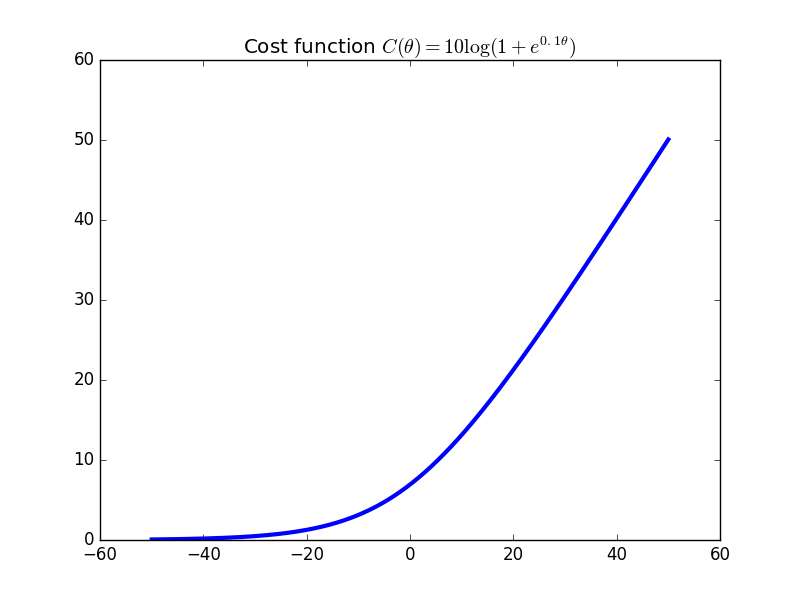
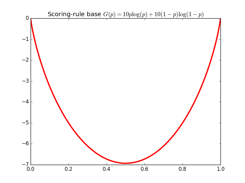
So the payoff to a participant updating from prediction $r$ to $r'$ is \begin{align*} & S(r',\omega) - S(r,\omega) \\ &= \left[ G(r') + dG(r')\cdot(\phi(\omega) - r') \right] - \left[ G(r) + dG(r)\cdot(\phi(\omega) - r) \right] . \end{align*} Now let $C$ be the convex conjugate of $G$: by properties of convex duality, $G(x) - dG(x)\cdot x = -C(dG(x))$ for all $x$. So \begin{align*} & S(r',\omega) - S(r,\omega) \\ &= \left[ dG(r')\cdot \phi(\omega) - C(dG(r')) \right] - \left[ dG(r)\cdot \phi(\omega) - C(dG(r)) \right] \\ &= (\theta_{r'} - \theta_r)\cdot \phi(\omega) - \left[ C(\theta_{r'}) - C(\theta_r) \right] \end{align*} where we used $\theta_x = dG(x)$. So we have shown that the agent's payoff can be rewritten in the cost function market form: she moves the market state from $\theta_r$ to $\theta_{r'}$, recieving share vector $d\theta = \theta_{r'} - \theta_r$ and paying $C(\theta_{r'}) - C(\theta_r)$.The cost function and convex conjugate for the single-dimensional logarithmic scoring rule market. Note how, as $\theta$ gets very negative, the slope -- which is price per share -- goes to zero. This is good: If everyone is selling, the probability of the event is probably close to zero. Similarly, as more and more people buy, the slope approaches one. The scaling factor $10$ controls how quickly prices change (see also Exercise 1).


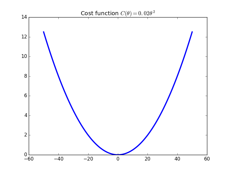
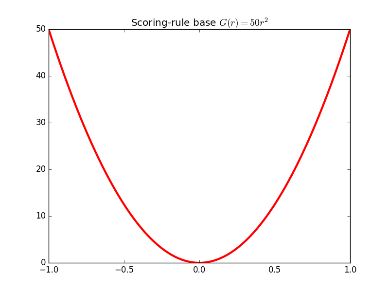
The cost function and convex conjugate for the single-dimensional quadratic scoring rule market. Here, the slopes (prices) increase/decrease without bound if enough shares are bought/sold. If it is impossible for the random variable to take a value larger than e.g. $50$, then it is irrational to continue buying once the price goes beyond $50$.


Duality details. What may seem like technical details of convex duality have very nice intuitive implications here.
First, we know that $S$ is only strictly proper if $G$ is strictly convex; otherwise, there is a "flat" portion of $G$ and reporting two different means, both on this flat portion, results in the same expected payoff. So while being truthful is optimal, agents can sometimes also optimize with certain misreports. Anywhere $G$ has a flat portion, its convex conjugate $C$ has a point of nondifferentiability. The slope $dG(r) = dG(r')$ for some points $r \neq r'$, which means that the set of subgradients of $C(dG(r))$ contains both $r$ and $r'$. (Remember, differentiability of a convex function at a point is equivalent to there only existing a single subgradient at that point.) What does a point of nondifferentiability mean for the cost function market? It means the instantaneous prices are not well-defined (hence the market prediction is ambiguous). Both $r$ and $r'$ are valid subgradients of $C$, hence valid predictions, at the share vector $\theta = dG(r) = dG(r')$. It means that an agent whose belief is in a certain set will not have any profitable trade to make when the current share vector is at $\theta$. Some directions will be too steep, others too shallow. This exactly corresponds to the original non-strict-properness of $S$.
Second, we know that if $G$ has a point of nondifferentiability, there are multiple choices of subgradient at that point which give a valid strictly proper scoring rule. By convex duality, such a point corresponds to a flat portion of $C$: this is a region where buying or selling shares does not change the current prices (slope). So prices can still be inferred from the current share vector, which is good; it just seems inefficient.
From the above discussion, we can see that it is desirable for both $G$ and $C$ to be both strictly convex and differentiable. In a future post, I'll talk more about axioms for prediction markets and how these correspond to properties of convex functions. We'll also discuss what you can do if you want your prediction market to reveal other properties of the distribution than linear ones (expectations).
Exercise 1 (scaling up markets). Given a scoring rule $S$, we can scale all participants' scores by using $S'(r,\omega) = bS(r,\omega)$ for any constant $b \gt 0$. Show that this modifies the corresponding cost function market from $C$ to $C'(\theta) = b C(\theta/b)$. (This is called the perspective transform.)
Exercise 2 (LMSR, scalar version).
Show duality between the following single-dimensional functions (i.e. interpret $p$ as a scalar in $[0,1]$): The log scoring rule with $G(p) = p \log(p) + (1-p)\log(1-p)$, and the cost function $C(\theta) = \log (1 + e^{\theta})$. This gives the so-called log market scoring rule.
Hint: introduce an auxiliary variable $y = e^{\theta}$ and show/use that $p=y/(1+y)$.
Exercise 3 (Quadratic, scalar version). Viewing $r,\theta$ as scalars, what is the convex $G$ and scoring rule associated with cost function $C(\theta) = 0.5 \theta^2$?
Exercise 4 (LMSR). Show duality between the general log scoring rule $G(p) = \sum_{\omega} p(\omega) \log p(\omega)$ and the cost function $C(\theta) = \log \sum_{\omega} e^{\theta_{\omega}}$.
Exercise 5 (Quadratic). Letting $r,\theta$ be vectors, what is the convex $G$ and scoring rule associated with cost function $C(\theta) = 0.5 \|\theta\|_2^2$?
References
(2003) Robin Hanson. Combinatorial information market design. Information Systems Frontiers.(2013) Jacob Abernethy, Yiling Chen, and Jennifer Wortman Vaughan. Efficient market making via convex optimization, and a connection to online learning. ACM Transactions on Economics and Computation.

