Topic D: Greedy Algorithms
- Section 1: Greedy Algorithms and Knapsack
- Section 2: Interval Scheduling
- Section 3: Minimum Spanning Trees
Section 1: Greedy Algorithms and Knapsack
This section introduces greedy algorithms and the knapsack problem. Greedy is an important general algorithmic paradigm to know, including its pitfalls.
Objectives. After learning this material, you should be able to:
- Explain the concept of a "greedy" algorithm.
- Recognize exchange arguments for greedy proofs of correctness.
- Recognize variants of the knapsack problem and prove when greedy is optimal, or provide a counterexample when it is not.
Definition and knapsack
We call an algorithm greedy if it takes a sequence of decisions that each look "locally" optimal at the current moment, without appearing to worry about global solution quality. To get the idea, let's look at an example.
Knapsack problem with uniform weights.
- Input: a list of items $i = 1,\dots,n$, with a value $v_i \geq 0$ for each. Also, an integer $W \geq 0$.
- Output: the subset of $W$ of the items that have the largest total value (i.e. sum of the values).
The problem's name comes from the image that our knapsack can fit at most $k$ items, and we want to put the highest-value total set in it. Before continuing, can you solve this problem?
A natural greedy algorithm is the following, which we'll state informally rather than in pseudocode:
- repeat W times:
- add the highest-value item remaining to the knapsack.
This algorithm is greedy: it makes a sequence of decisions that are optimal in the moment, i.e. taking the highest-value item available. But it turns out to be globally optimal too. This is probably not surprising in this case, but proving it will introduce some important ideas.
The greedy algorithm is correct, i.e. returns the subset of size $W$ with highest total value.
We use an exchange argument, which involves showing that any other solution can be improved by swapping or exchanging part of its solution out for the greedy algorithm's solution.
Let us re-name the items so that $v_1 \geq v_2 \geq \cdots \geq v_n$. The greedy algorithm's solution set is $\{1,\dots,W\}$ with value $\sum_{j=1}^W v_j$.
To prove it's optimal, consider any other solution set $S$, a subset of $\{1,\dots,n\}$ of size at most $W$. Suppose $i > W$ and $i \in S$. Then there must be some item $j \in \{1,\dots,W\}$ such that $j \not\in S$. Notice that $j < i$, so $v_j \geq v_i$.
Let's make a swap: remove $i$ from $S$ and add $j$ instead. The value of $S$ goes up by $v_j - v_i \geq 0$. So the value of $S$ only improves.
Now let's just repeat this process over and over. Eventually, $S = \{1,\dots,W\}$ because we swap in all of the first $W$ items that were missing. The value of $S$ only goes up each time. So the greedy solution set is optimal.
While there's no universal definition of greedy algorithms, many of them share the above components:
- The algorithm's job is to construct a solution set.
- The goal is to maximize some total "value" of the solution across the entire set (a global objective).
- The algorithm proceeds by "greedily" choosing an item that looks the best "locally" in the current moment, and repeating this until the solution set is constructed.
We will see several other examples, but first, let's look at variants of the problem where greedy fails.
Failure of greedy algorithms
For algorithm designers, almost as important as designing correct algorithms is identifying failure points of incorrect ones. Let's look at a variant of knapsack where the greedy algorithm fails.
Knapsack problem.
- Input: a list of items $i = 1,\dots,n$, with a value $v_i \geq 0$ for each and a weight $w_i \geq 0$ for each. Also, a weight limit $W \geq 0$.
- Output: the subset of the items that have the largest total value (i.e. sum of the values), whose total weight is at most $W$.
Let's do an example.
| Item $i$ | Value $v_i$ | Weight $w_i$ |
|---|---|---|
| 1 | 10 | 1 |
| 2 | 15 | 3 |
| 3 | 7 | 2 |
Suppose the weight limit is $W = 4$. Our greedy algorithm is the same as before, but must respect the weight limit: add the highest value item, then the next, and so on. If an item doesn't fit in our weight limit, skip it, and once no more items fit, we're done.
On the above instance with a weight limit $W=4$, what output does this greedy algorithm produce? Is that optimal?
Solution.
Greedy first takes item 2, which has a value of 15. It has weight 3. It then takes item 1, with a value of 10 and weight of 1. The total value is now 25 and total weight is 4. Now, we can't take any more items and stop.
Yes, 25 is the optimal possible solution for this instance. We can't fit all three items, and we have the two most valuable items.
Now comes a key question. Can you solve it?
Give a different weight limit $W$ so that, on the above instance, the greedy algorithm fails to find the optimal solution. Explain how.
Solution.
We can use $W=3$. In this case, greedy will take item 2 and then stop, for a total value of 15. But we could take items 1 and 3 instead for a total value of 17, while still having a weight of 3.
It's worth reflecting on why greedy failed here. We needed to take into account the resources being used up (i.e. weight) by the items, not just their value. Here is another exercise.
Consider the following greedy algorithm for knapsack: always take the item with smallest weight, until the knapsack is full (i.e. no more items fit in the weight limit). Is this algorithm always optimal? If so, give a proof. If not, give a counterexample and explain.
Example solution.
It is not always optimal. There are many possible counterexamples, but the general idea is to make low-weight items have very low values.
| Item $i$ | Value $v_i$ | Weight $w_i$ |
|---|---|---|
| 1 | 1 | 1 |
| 2 | 1 | 1 |
| 3 | 10 | 2 |
Suppose the weight limit is $W=2$. This greedy algorithm will take items 1 and 2, for a total value of 2. But the optimal solution is to take just item 3, for a value of 10.
Section 2: Interval Scheduling
This section discusses another set of problems where greedy algorithms can often be optimal.
Objectives. After learning this material, you should be able to:
- Define the interval scheduling problem and execute greedy algorithms for it.
- Prove that greedy is correct via an exchange argument.
- Decide for which variants greedy is not correct and provide counterexamples.
The interval scheduling problem
Interval scheduling is a problem where we have a resource available over time, and a set of requests to use the resource. An example would be a server and requests to use the server to run heavy computations; another would be a soccer field and requests to schedule games.
Each request will have a start and end time. Our goal is to schedule as many requests as possible, but we are not allowed to have overlapping requests.
Interval scheduling problem:
- Input: a list of requests $i=1,\dots,n$. Each has a start time $s(i)$ and an end time $t(i)$, which we can assume are integers.
- Output: a subset $S$ of the requests that we want to schedule. The subset must not be overlapping, i.e. only one request may be executing at any given time. The goal is to maximize the size of the subset.
As always when you see a new problem, it's good to do some examples.
Given the following instance of interval scheduling, what is the optimal solution? Are there more than one?
| $i$ | $s(i)$ | $t(i)$ |
|---|---|---|
| 1 | 0 | 40 |
| 2 | 10 | 30 |
| 3 | 35 | 80 |
| 4 | 50 | 65 |
| 5 | 75 | 100 |
Hint: draw a diagram like this...
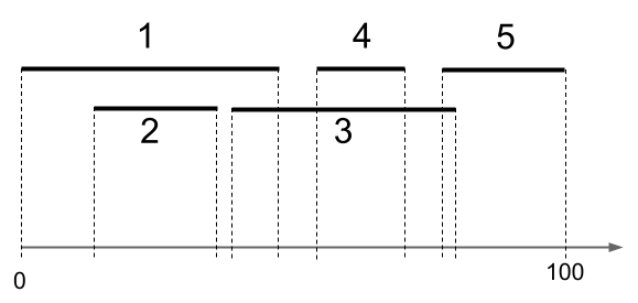
Solution.
The maximum number of requests we can schedule is three. There are two optimal solutions: $\{1,4,5\}$ and $\{2,4,5\}$. In either case, there are no overlaps and we schedule 3 different requests. There is no way to schedule four or five requests.
First greedy attempt
There are many possible greedy strategies here. Let's brainstorm a few greedy algorithms. Can you think of any?
A few to get started.
- Always pick the smallest interval (that doesn't overlap with any that you've picked so far).
- Always pick the an interval that overlaps with as few others as possible.
Can you think of other greedy strategies?
It turns out that a number of natural-looking greedy strategies don't actually work. Let's try disproving one.
Using a counterexample, prove that the algorithm that always picks the smallest valid interval is not optimal.
Example solution.
There are many possible answers; here's one.
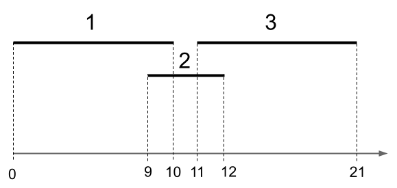
Figure: 3 intervals. We have $s(1) = 0, t(1) = 10$, meaning that the first interval starts at time zero and ends at time 10. We have $s(2) = 9, t(2) = 12$. And $s(3) = 11, t(3) = 21$.
The optimal solution is $\{1,3\}$, giving us two intervals. But the greedy-by-smallest algorithm would first pick interval 2. Then it would not be able to pick any more intervals, so it would have a solution size of just one interval.
A correct greedy algorithm
It turns out this problem does have a greedy algorithm that optimally solves it, but we have to be a bit clever about what to be greedy with. Here's the algorithm:
- Select the interval that is scheduled to finish first, i.e. has minimum $t(i)$. Remove from consideration any intervals that overlap with it.
- Repeat until no intervals remain.
The above algorithm, greedy by first finish time, is correct for interval scheduling.
We will use an exchange argument. Suppose greedy selects the requests $S = \{ i_1,\dots,i_k \}$, in order of start time and finish time. Consider any other feasible solution (meaning no overlaps), $R = \{j_1,\dots,j_r\}$, also in order of start and finish time. We want to show that $k \geq r$, that is, greedy selects at least as many requests.
First, because of how greedy works, $t(i_1) \leq t(j_1)$. So we can remove $j_1$ from $R$ and add $i_1$ and $R$ is still feasible, and the number of requests has not changed. Next, consider $j_2$. We have $s(j_2) > t(j_1) \geq t(i_1)$. So greedy could have added $j_2$ next. But greedy added $i_2$. Therefore, because of how greedy works, $t(i_2) \leq t(j_2)$. So we can remove $j_2$ from $R$ and add $i_2$ and $R$ is still feasible, and the number of requests has not changed.
We repeat this argument until the very end. Suppose for contradiction that $k < r$, so after we exchange $i_k$ into $R$ for $j_k$, there still remains some request $j_{k+1}$. If this were possible, then greedy would have added $j_{k+1}$ to its solution, since it is feasible (we must have $s(j_{k+1}) > t(j_k) \geq t(i_k)$). This is a contradiction. We conclude $k \geq r$.
Section 3: Minimum Spanning Trees
This section discusses a fundamental problem in graph theory and uses greedy algorithms to solve it.
Objectives. After learning this material, you should be able to:
- Define the minimum spanning tree (MST) problem.
- Use properties of spanning trees to solve related problems.
- Execute Prim's and Kruskal's algorithms.
Spanning trees
First, we need to recall the definition of a tree. Previously in this class, we defined rooted trees. We can think of a tree as a rooted tree, where we deleted all information about which node is the root and which nodes are children of which. Here is a formal definition:
An undirected graph $T = (V,E)$ is a tree if it is connected and has no simple cycles.
Remember that connected means there is a path from every vertex to every other vertex. A simple cycle is a path of length at least three that starts and ends at the same vertex and does not repeat edges. Here is a nice fact about trees.
Any tree on $n$ vertices has exactly $n-1$ edges.
By induction on $n$. The base case is $n=1$. A graph with one vertex will have no edges (we generally assume that self-loops are not allowed), so the formula is satisfied.
Now let $n \geq 2$ and suppose that any tree on $n' < n$ vertices has exactly $n'-1$ edges. Consider a tree on $n$ vertices. Let us delete any edge $\{u,v\}$. We first claim this disconnects the graph into two disjoint trees. First, deleting an edge cannot have created a cycle. Next, it is partitioned into two connected components: originally, every vertex was reachable from $u$, and the path from $u$ either included the edge $\{u,v\}$ or not. If so, the vertex is still reachable from $v$ after the disconnection, and if not, it is still reachable from $u$ after the disconnection. Further every vertex is in either one case or the other, but not both, as otherwise there would be a cycle in the original graph involving a path to the vertex from $u$ and from $v$, along with the edge $\{u,v\}$. So the graph is partitioned into two disjoint connected acyclic graphs, i.e. trees.
The trees have $n_1,n_2 \geq 1$ vertices with $n_1 + n_2 = n$. By inductive hypothesis, they have $n_1-1$ and $n_2-1$ edges. Adding $\{u,v\}$, the total number of edges in our original tree is $n_1 - 1 + n_2 - 1 + 1 = n-1$.
Next, we can define a spanning tree. Intuitively, given a connected, undirected graph, we may want to delete as many edges as possible while keeping the graph connected. The minimum set of edges we need to keep form a tree, called a spanning tree.
In an undirected graph $G = (V,E)$, a spanning tree is a tree $T = (V,E')$ where $E' \subset E$. In other words, it is a subgraph of the original graph that includes all the vertices and is a tree.
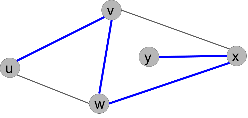
Give a spanning tree of this graph.
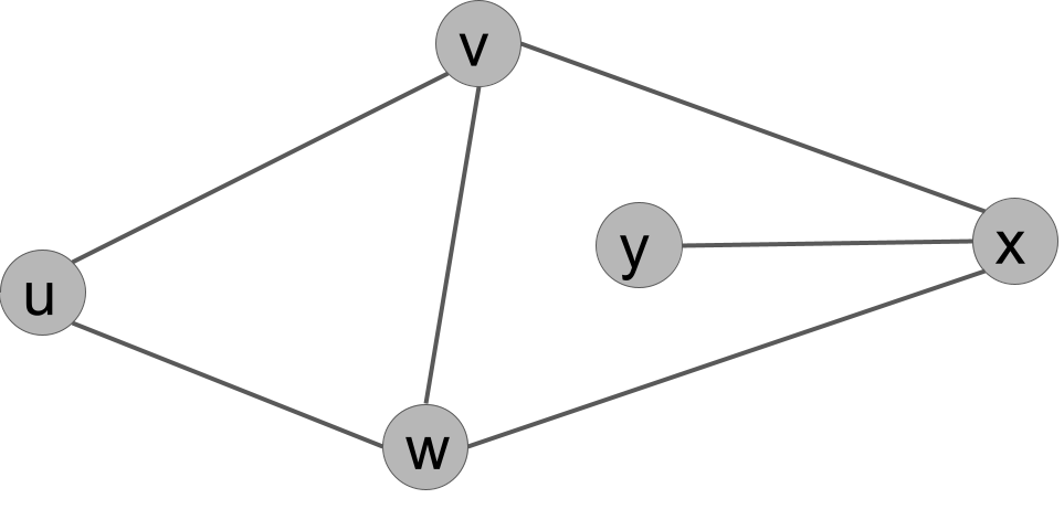
Example solution.
There are several solutions. Because there are 5 vertices, any subset of 4 edges that keep the graph connected form a spanning tree. Here is one (the thick blue edges):
Minimum spanning tree (MST) and reverse-deletion
In the minimum spanning tree problem, our graph is undirected and weighted. We assume the weight $wt(u,v)$ on each edge is positive.
Minimum spanning tree (MST) problem:
- Input: a connected, weighted, undirected graph. We assume for simplicity that all edge weights are distinct.
- Output: a spanning tree where the sum of the edge weights is as small as possible.
This problem can arise in many contexts. Picture a communication network, such as a network of computers. We want to ensure that the network is connected so that every node can send a message through the network to every other node. However, maintaining all of the links (edges) may be costly. We want to reduce the number of links to the minimum-cost set needed in order to maintain communication.
It is worth noting the following point. Can you prove it?
The minimum-cost set of edges that keep the graph connected will always form a tree.
Proof.
Suppose we have a set of edges where the graph is connected, but not a tree. Then there is a cycle. If we delete one edge $\{u,v\}$ from the cycle, the graph is still connected, because we can still get from every node on the cycle to every other node. And deleting the edge has reduced the total cost of this set of edges. We can repeat this argument as long as the graph has cycles until we end with a connected, acyclic graph: a tree.
This observations gives an idea for our first greedy algorithm for MST.
The Reverse-Deletion Algorithm:
- Sort the edges from largest weight to smallest.
- Go through the list, deleting each edge unless doing so disconnects the graph.
Correctness
For correctness, as with Dijkstra's algorithm, we need a key fact about the problem. Here is the fact:
For any simple cycle in the graph, the maximum-weight edge in the cycle is not part of any minimum spanning tree.
Let $v_1,\dots,v_k=v_1$ be a simple cycle and suppose without loss of generality that $\{v_1,v_2\}$ is the maximum-weight edge in the cycle. Suppose we have a spanning tree $T$ containing $\{v_1,v_2\}$. We prove it is not a minimum spanning tree.
Delete $\{v_1,v_2\}$ from the tree, leaving us with two disjoint trees, say $T_1$ containing $v_1$ and $T_2$ containing $v_2$. Adding any edge between a vertex in $T_1$ and a vertex in $T_2$ will connect the trees into a spanning tree again. And in the original graph, there is a path $v_2,\dots,v_{k-1},v_1$. Since the start is in $T_2$ and the end is in $T_1$, at least one of these edges crosses over. And it must have smaller weight than $\{v_1,v_2\}$, so adding it results in a spanning tree with smaller weight than $T$, so $T$ could not have been a MST.
The Reverse-Deletion algorithm correctly produces a MST.
Suppose that deleting an edge does not disconnect the graph. Then that edge must have been part of a simple cycle, because there is still a path between its endpoints. So by the Proposition, that edge cannot have been part of any minimum spanning tree. Therefore, if we delete it, a minimum spanning tree of the resulting graph is also a MST of the original graph. Now we just need to note that Reverse Deletion continues until the set of remaining edges is a spanning tree, because otherwise, by definition, there is a cycle and some edge could be deleted. Since it stops at a spanning tree, that spanning tree is a MST of the original graph.
Kruskal's and Prim's algorithms
We will look at two other correct greedy algorithms for minimum spanning tree. They both rely on the following key fact.
Let $R,S$ be any cut in the graph, meaning a partition of the graph into two disjoint sets of vertices. Let $\{u,v\}$ be the minimum-cost edge that crosses the cut. Then every MST of the graph contains $\{u,v\}$.
Consider any spanning tree of the graph that does not contain $e$. We will show it is not a minimum spanning tree.
Suppose without loss of generality that $u \in R$ and $v \in S$. Because it's connected, there is a path in the spanning tree from $u$ to $v$. This path "crosses" the cut at some point, i.e. includes some edge $\{u',v'\}$ with $u' \in R$ and $v' \in S$. Let us delete $\{u',v'\}$ and add $\{u,v\}$. By assumption, the total cost of the edges has decreased. Is it still a spanning tree? It is still connected, because there is now a path from $u'$ back to you, across $\{u,v\}$ to $v$, and then to $v'$. So any prior path that used $\{u',v'\}$ can be transformed into a path that uses $\{u,v\}$. Similarly, there are no cycles, because if there is a cycle including $\{u,v\}$ now, we could transform it into a cycle that uses $\{u',v'\}$ in the original graph. (The cycle might not be simple, but we can turn it into a simple cycle from there.)
This fact suggests an algorithm that is a sort of mirror to the Reverse Deletion algorithm.
Kruskal's algorithm:
- Sort the edges from smallest weight to largest.
- Go through the list, adding each edge to the graph unless doing so creates a cycle.
Kruskal's algorithm outputs a minimum spanning tree.
When we add an edge $\{u,v\}$, let $R$ be the set of vertices reachable from $u$ along edges added so far, and let $S$ be the remaining vertices. Note that adding any edge that crosses the cut would not create a cycle, since currently no edges cross the cut. Therefore, $\{u,v\}$ must be the minimum-weight edge that crosses this cut, since we are adding edges in order. So by the Proposition, every minimum spanning tree contains $\{u,v\}$, so we are safe to add it to our solution. Now we just need to show that Kruskal's produces a spanning tree. The output doesn't have cycles by definition. But it is a tree, since if it were disconnected at the end, there would be some edge that could have been added (as the original graph was connected), a contradiction. So Kruskal's produces a spanning tree, and it is minimum because it only contains edges that are in every MST.
A small complaint about Reverse-Deletion and Kruskal's is that they are not clearly efficient. First, sorting the edges at the beginning takes $O(m \log(m))$ time, and $m$ can be quite a bit larger than $n$. Second, checking in every loop for whether a cycle has been created takes a significant amount of time. A straightforward approach is to use BFS or DFS each time to check for a cycle. However, doing this every loop is a somewhat slow process. (For Kruskal's, the time complexity can be improved significantly with the union-find data structure, but we won't cover that here.) Can we do better? Yes: here is Prim's algorithm.
Prim's algorithm:
- Pick any vertex $u$, and add it to our set $R$.
- Add the minimum-cost edge $\{u,v\}$ attached to $u$ to our solution, and add its other endpoint $v$ to $R$.
- Continuing, add the minimum-cost edge leaving $R$ to our solution and add its other endpoint to $R$.
- Stop when $R = V$, the set of all vertices.
Prim's algorithm outputs a minimum spanning tree.
At every step, we add the minimum-cost edge that crosses a cut in the graph, where the cut is $R$ and $V \setminus R$. So by the Proposition, every edge we add must be part of every minimum spanning tree. And we certainly produce a spanning tree, because we never create a cycle and we eventually connect all vertices.
Running time analysis of Prim's algorithm
To analyze running time, we should have a more precise definition of the algorithm. In fact, it will look extremely similar to Dijkstra's algorithm. As with Dijkstra's, we will use a Priority Queue.
// Prim's algorithm
1  prim(G):
2      // G = (V,E) is a weighted, undirected, connected graph
3      Q = new Priority Queue
4      for all vertices u:
5          best_weight[u] = infinity
6          best_edge[u] = null
7          marked[u] = false
8          Q.insert(u, infinity)
9      let s be any vertex of G
10     Q.update(s, 0)
11     let F = empty list        // edges of the spanning tree
12     while Q.size() > 0:
13         u = Q.pop_smallest()
14         marked[u] = true
15         F.add(best_edge[u])   // does nothing if best_edge[u] is null
16         for v in N(u):
17             if not marked[v] and wt(u,v) < best_weight[v]:
18                 best_weight[v] = wt(u,v)
19                 best_edge[v] == {u,v}
20                 Q.update(v, wt(u,v))
21     return (V, F)
To understand the pseudocode, see if you can answer this question (you will want to take another look at Dijkstra's).
What is the key difference between Prim's and Dijktra's algorithms? How do these differences result in one solving MST while the other solves shortest paths?
Solution.
The key difference is that in the array and priority queue, Dijkstra tracks the smallest total distance from the source to a given vertex. Prim tracks the smallest edge to the vertex from any previously-visited vertex. This means that Dijkstra keeps popping vertices with smallest distance from the source, but Prim keeps popping vertices that have the smallest edge to the current connected component. So Dijkstra is finding paths from $s$ that are as short as possible, while Prim is connecting a tree as cheaply as possible.
The running time of this implementation is essentially identical to Dijksta's. If we use a Fibonacci heap, we obatin the following analysis, which is the same as in Dijkstra's.
| Operations | Total time complexity with F. heap |
|---|---|
| $O(n)$ calls to Q.insert() | $O(n)$ |
| $O(n)$ calls to Q.pop_smallest() | $O(n \log(n))$ |
| $O(m)$ calls to Q.update() | $O(m)$ |
The result is a running time of $O(m + n \log(n))$, just as with Dijkstra's algorithm. We also should note that we have $O(n + m)$ operations otherwise, but this will be dominated in big-O by the complexity of the heap operations.