Topic C: Graph Traversal
Section 1: Graphs and Trees
This section introduces graphs and graph terminology. Many, many computational problems are modeled as problems to do with graphs, as we will soon see.
Objectives. After learning this material, you should be able to:
- Recall and apply definitions such as graph, neighbors, degree, paths, etc.
- Constrast the performance of the adjacency matrix and the adjacency list representations of a graph.
- Recall and apply definitions for trees, including root, children, height, etc.
Graphs, formally
As you know, graphs represent a set of objects (the vertices) and relationships between the objects (the edges). Grahps are used to model many settings, such as:
- Road networks
- Computer networks
- Social networks (friendship graphs)
- Web pages and hyperlinks
- Financial networks
- Biological systems
- States of a system and transitions between states
Formally:
A graph $G = (V,E)$ consists of a set of vertices (also called nodes), $V$, and a set of edges, $E$. The graph is directed if each edge $e = (u,v)$ represents an ordered pair, where the edge goes from $u$ to $v$. The graph is undirected if each edge $e = \{u,v\}$ represents an unordered pair, where the edge equally connects $u$ to $v$ and $v$ to $u$.
The number of vertices is $|V|$ and is usually called $n$. The number of edges is $|E|$ and is usually called $m$.
For example, in a social network, the vertices are people, and there is an edge $(u,v)$ if person $u$ is "following" person $v$. We also recall these useful graph concepts.
- A neighbor of $u$ in an undirected graph is a vertex $v$ with whom $u$ shares an edge. We sometimes use $N(u)$ to denote the set of neighbors of $u$.
- The degree of $u$ in an undirected graph is the number of its neighbors.
- An out-neighbor of $u$ in a directed graph is a $v$ for which $(u,v)$ is an edge. Similarly, an in-neighbor is a $v$ for which $(v,u)$ is an edge.
- The out-degree is the number of out-neighbors; similarly for in-degree.
- A path in a graph is a list of vertices $v_1,\dots,v_k$ where there is an edge from each vertex to the next. In a directed graph, the edges must "point" forward. The length of the path is the number of edges, i.e. $k-1$.
- A cycle in a graph is a path $v_1,\dots,v_k$ of length at least $2$ where $v_k = v_1$, i.e. we end where we started.
- Often, when we say cycle, we really mean simple cycle, which is a cycle that does not have any repeated edges or vertices. It is always good to double-check whether simple cycle is meant.
Test your understanding of the terminology:
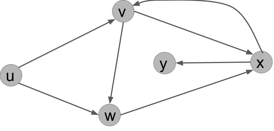
For the following directed graph, answer these questions:
- List all the edges in the graph.
- What is the out-degree of $u$?
- Name all of the in-neighbors of $v$.
- Is $(u,v,w,x,y)$ a path in the graph?
- Is $(u,w,y,x,v)$ a path in the graph?
- What is a cycle in the graph?
Solution.
- $(u,v), (u,w), (v,w), (v,x), (w,x), (x,v), (x,y)$.
- $2$.
- $u$ and $x$.
- Yes.
- No: there is no edge from $y$ to $x$.
- There are several answers. One cycle is $v,w,x,v$. This is a cycle because it is a path (a list of vertices where an edge connects each vertex to the next) and the last vertex in the list equals the first.
Here is a fun fact that will be useful later:
In an undirected graph, the sum of the degrees of the vertices is equal to twice the number of edges.
Every edge has two endpoints, e.g. $u$ and $v$. If we sum over the vertices the degree of each vertex, then for $u$, the edge is counted once, and for $v$, the edge is counted once. Therefore, each edge is counted twice in total.
Adjacency matrix representation
How do we write a graph down for a computer to work with? There are two main ways. The first is called the adjacency matrix representation. For a graph with $n$ vertices, it is an $n \times n$ matrix, where a $1$ in the $(u,v)$ entry represents that there is a directed edge from $u$ to $v$. If the graph is undirected, then the matrix is symmetric, i.e. there is $1$ at position $(u,v)$ if and only if there is a $1$ at position $(v,u)$.
For the example graph above, here is its adjacency matrix:
| u | v | w | x | y | |
|---|---|---|---|---|---|
| u | 0 | 1 | 1 | 0 | 0 |
| v | 0 | 0 | 1 | 1 | 0 |
| w | 0 | 0 | 0 | 1 | 0 |
| x | 0 | 1 | 0 | 0 | 1 |
| y | 0 | 0 | 0 | 0 | 0 |
The adjacency matrix data structure has the following important characteristics:
- Space: the size of the data structure is $n^2$ regardless of the number of edges.
- Edge query: checking whether an edge $(u,v)$ exists or not is an $O(1)$ time operation. We can just jump to the appropriate location in the list and check.
- Neighbors query: getting the list of out-neighbors of a vertex $u$ is an $O(n)$ time operation, because we need to scan the entire $u$ row of the matrix to check for all the neighbors.
Adjacency list representation
The second main way to write down a graph is as an adjacency list. This consists of an array where, for each vertex, we list all of its out-neighbors.
For the example graph above, here is its adjacency list:
| vertex | out-neighbors |
|---|---|
| u | v, w |
| v | w, x |
| w | x |
| x | v, y |
| y | $\quad$ |
The adjacency list data structure has the following characteristics:
- Space: the size of the data structure is $O(n + m)$, where $n$ is the number of vertices and $m$ is the number of edges.
- Edge query: checking whether an edge $(u,v)$ exists is no longer constant time, but involves scanning through the list associated with $u$ for the presence of $v$.
- Neighbors query: getting the list of out-neighbors of a vertex is now $O(1)$ time, because it is already written down for us.
We can see that the adjacency list might be much smaller to store than the adjacency matrix and can be faster if we need to iterate through the neighbors of vertices. However, the adjacency matrix is faster for looking up existence of given edges.
Weighted graphs
A weighted graph is a graph where, for each edge $(u,v)$, we are given a weight $w(u,v) \in \mathbb{R}$. With adjacency matrices, we can represent the weight directly in the entry of the matrix, replacing $1$ with the actual weight. Depending on the application, we may treat a weight of zero or a weight of infinity as "edge does not exist". With adjancency lists, we can simply store the weights in the lists next to the corresponding neighbor.
In a weighted graph, the length of a path is now the sum of the weights along the path. Here is an example weighted graph:

In this graph, the path $u,v,w,x$ has length $3 + 8 + 5 = 16$.
Trees
A tree is a special type of graph. We will define trees inductively.
A tree is a graph organized as follows. There is a vertex $r$ called the root.
- $r$ by itself with no edges is a tree.
- Given a set of trees $T_1,\dots,T_k$ with roots $v_1,\dots,v_k$ respectively, the graph produced by connecting $r$ to each of $v_1,\dots,v_k$ is a tree. In this case, we say $r$ is the parent of each $v_i$, which is a child of $r$.
Technically, this is called a rooted tree. If we form a rooted tree, then take away the designation of which node is the root node, we are left with a regular old tree. We will come back to those later in the course, but focus on rooted trees for now.
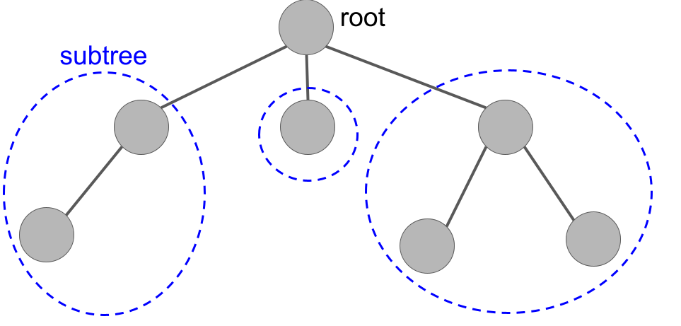
A tree formed by taking three "subtrees" and connecting them to a new root.
Let us practice induction by proving an important fact.
A tree with $n$ vertices always has $n-1$ edges.
The base case is a tree with $n=1$ vertex, which has $0=n-1$ edges as required.
For the inductive case, let $n \geq 2$ and suppose all trees with $t < n$ vertices have $t-1$ edges. A tree on $n$ vertices is formed by a root $r$ connected to a set of trees $T_1,\dots,T_k$. These have a total of $n-1$ vertices, since adding the root makes $n$. Therefore, they have a total of $n-1-k$ edges, because each tree contributes one fewer edges than vertices by inductive hypothesis. Now we need to add the edges between $r$ and the roots of each of the subtrees, which adds $k$ edges. The total is $n-1$.
We recall some more tree terminology:
- A vertex with no children is called a leaf.
- The height of a tree is the length of the longest path from the root to a leaf.
- An ancestor of a vertex is a parent, parent of a parent, etc. all the way back up to the root.
- A descendent of a vertex is a child, child of a child, etc.
Section 2: Exploring Graphs
In this section, we'll learn about algorithms for exploring graphs by hopping from vertex to neighboring vertex.
Objectives. After learning this material, you should be able to:
- Describe search trees produced by exploring a graph.
- Execute depth-first search and breadth-first search on a graph and recall their runtime analyses.
- Contrast the search trees that can be produced by DFS versus by BFS.
Depth-first search
One of the most basic and important tasks to do on graphs is to explore them: starting from a known vertex, pick a neighbor, go to that neighbor, and repeat. In this way, we learn how vertices are related by distance. For example, we can learn if a graph is connected -- can every vertex be reached from every other vertex?
We'll start with one of the most common exploration methods, depth-first search (DFS). DFS is named "depth-first" because it explores as far as possible before "backtracking". We will compare it to breadth-first search later.
// Algorithm 1: Depth-First Search
1 DFS(G, s):
2     // G = (V,E) is an undirected graph and s is a vertex
3     for each v in V:
4         let marked[v] = False
5     explore(s)
// Subroutine 1: explore recursively
1 explore(v):
2     set marked[v] = True
3     print v                     // or do other useful work with v
4     for each neighbor w of v:
5         if not marked[w]:
6             explore(w)
Execute DFS(G,u) on this graph. In what order does it print the vertices?
Hint: there are multiple correct answers, depending on in which order the neighbors of each vertex are listed.
Solution.
Here is one answer: u v x y w.
To picture the answer, you can also draw on each vertex the order in which it is marked.

We can also represent the calls to explore() like this:
1 explore(u)
2     explore(v)
3         explore(x)
4             explore(y)
5         explore(w)
This represents the following order of calls to explore. We explore u, which steps to v, which steps to x, which steps to y. At that point, because y has no outgoing edges, the call explore(y) finishes and we backtrack to x. It has another out-edge to v, but v is already marked. So the call explore(x) finishes, and we backtrack to v. It has another out-edge to w, which is not yet marked, so we call explore(w). This call does nothing because w's only out-neighbor is already marked. Then the call to explore(v) is finally done, and we go back to u. It has another out-neighbor w, but w is already marked by now, so we're done.
Notes. If the graph is fully connected, then we will eventually call explore() on every vertex. However, if the graph is not connected, then DFS(G) will only explore nodes reachable from $s$.. You can see this by trying the code on small examples of connected and disconnected graphs.
In many applications, we would replace line 3 of explore(v) with some useful operation involving vertex v. As long as that operation takes constant time, the complexity analysis below will still apply. If not, the analysis below could be modified accordingly.
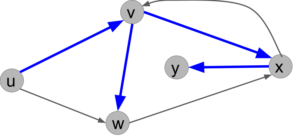
Search trees
Given a graph, the execution of DFS produces a search tree, which we define as follows. The root is the first vertex $r$ on which we call explore(r). Then, for each node $v$, its children are all the nodes $w$ where we call explore(w) from within the call to explore(v).
For example, for the solution of the exercise above, we get the following search tree (the blue edges), where the root is $u$.
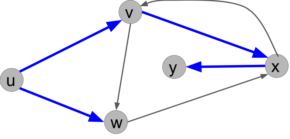
Explain why the following search tree can not be obtained by running DFS(u), no matter what order ties are broken in.

Solution.
From u, we either call explore(v) or explore(w) first. If we call explore(v) first, then v would always call explore(w) before u does, so the tree would have to have the edge (v,w) and not the edge (u,w). On the other hand, if we call explore(w) first, then that call would immediately call explore(x) because x would be unmarked. So the edge (w,x) would have to be present in the tree. Either way, the given search tree is not possible.
Runtime analysis
We now analyze the runtime of DFS. This is an interesting problem because it is recursive, but it is not a divide-and-conquer algorithm. We will need to carefully track the resource usage over the course of the algorithm. Recall that $n$ is the number of vertices in $G$ and $m$ is the number of edges.
First, we need to settle on an input representation. We will choose an adjacency list. This implies that we can iterate over the neighbors $N(v)$ of $v$ in time $O(|N(v)|)$, i.e. the number of neighbors. Recall that if we were using an adjacency matrix, then iterating through the neighbors of $v$ would take $O(n)$ time regardless of the number of neighbors.
Now we prove some useful facts.
For each vertex $u$ in the graph, explore(u) is called exactly once.
Each vertex $u$ starts unmarked (meaning that marked[u] is False) and is set to marked immediately when explore(u) is called. Since every call to marked(u) is protected by a statement of if not marked[u], explore(u) can only be called once. But the for loop of line 4 of DFS ensures that explore is called for every vertex.
Each call to explore(u) does at most $3|N(u)| + 2$ steps, not counting recursive calls to explore().
Lines 2 and 3 take $1$ step each. Thanks to the adjacency list, the for loop over the $|N(u)|$ neighbors can be iterated through in constant time per neighbor. So the for loop takes $3$ steps per loop, not counting work done within recursive calls. This gives a total of $3|N(u)| + 2$.
The call to DFS(G) does $O(n)$ work, not counting the call to explore().
The for loop executes $n$ times and does $O(1)$ work per loop.
Finally, we can analyze the runtime.
DFS runs in time $O(n + m)$, where $n$ is the number of vertices and $m$ is the number of edges.
The total work can be counted as the work done within DFS(G), which is called once, plus the sum of the work done in all the calls to explore(). We have shown that DFS(G) does $O(n)$ work internally. We have:
We used that the sum of the number of neighbors in the graph is equal to twice the number of edges. Adding this to the $O(n)$ used by DFS, we get a total running time bound of $O(n + m)$.
Application: connectivity
DFS has many applications, but here is a simple one. Recall that an undirected graph is connected if there is a path from any vertex to any other vertex. Otherwise, it is disconnected.
// Algorithm 2: Connectivity
1 is_connected(G):
2     pick any vertex s of G
3     DFS(G, s)
4     for each vertex v in G:
5         if not marked[v]:
6             return false
7     return true
We simply walk the graph from any starting vertex using DFS. When it returns, we check if every vertex has been marked; if so, we return true (the graph is connected), but if there is an unmarked vertex, we return false.
What is the running time of is_connected(G)?
Solution.
It is $O(n + m)$, because it calls DFS, which is $O(n + m)$, and then does $O(n)$ work itself due to the for loop.
The algorithm is_connected(G) is correct for connectivity.
First, we have to show it's correct on any connected graph. If $G$ is connected, then for every $v$, there is a path from $s$ to $v$. The path looks like $s, u_1, u_2, \dots, u_k, v$. Well, since there is an edge from $s$ to $u_1$, we know that we call explore(u1) at some point. Since there is an edge from $u_1$ to $u_2$, we know we call explore(u2) at some point. Repeating, we eventually call explore(v). So $v$ is marked. This holds for every $v$, so is_connected(G) will be correct.
Now suppose $G$ is not connected. Then there are two vertices $v,w$ with no path between them. That means that $s$ cannot have a path to both of them, since otherwise there would be a path between them that goes through $s$. So there is some vertex, call it $v$, with no path to $s$. But DFS(G, s) only explores $s$, vertices with an edge from $s$, vertices with an edge from those vertices, etc. So it only explores a vertex if there is a path to that vertex from $s$. So $v$ is never marked, so is_connected(G) will be correct.
Notice that in the proof, it didn't matter what vertex $s$ we started from: the proof works for any $s$.
Breadth-first search
Now we'll look at a different way to explore graphs, breadth-first search (BFS). Unlike DFS, in BFS we first look at all neighbors of the starting node, then all of its neighbors, and so on.
BFS will need a data structure called a queue, more specifically a First-In-First-Out (FIFO) queue. This data structure can be pictured as a list that supports the following operations:
FIFO Queue:
| Operation | Time complexity | Meaning |
|---|---|---|
| append$(v)$ | $O(1)$ | add $v$ to the end of the list |
| pop$()$ | $O(1)$ | remove the first item of the list and return it |
| size$()$ | $O(1)$ | return current size of list |
This data structure can be implemented e.g. with a linked list. Given a FIFO queue, BFS can be defined as follows:
// Algorithm 2: Breadth-First Search
1  BFS(G, s):
2      // G = (V,E) is an undirected graph and s a vertex
3      for each u in V:
4          let marked[v] = False
5      let Q = new FIFO_Queue
6      Q.append(s)
7      set marked[s] = True
8      while Q.size() > 0:
9          let u = Q.pop()
10         print u                      // or do other useful work with v
11         for each neighbor v of u:
12             if not marked[v]:
13                 Q.append(v)
14                 set marked[v] = True
We can think of BFS as expanding outward in a wave, or in "layers". The zeroth layer is the start vertex, $s$. The next layer consists of all neighbors of $s$. These are all inserted into the queue before any other vertices, so they are popped from the queue before others as well. The next layer are all "neighbors of neighbors", and so on.
Execute BFS(G,u) on this graph. In what order does it print the vertices?
Example solution.
There are multiple solutions depending on the ordering of the vertices, but here is one: $u, v, w, x, y$. In other words, the vertices are popped from the queue in this order:

- First, the start vertex, $u$, is popped. Its two out-neighbors are $v$ and $w$, and both are unmarked. It places them in the queue, let's suppose in the order $v,w$.
- Then, $v$, is popped. Its two out-neighbors are $x$ and $w$. First, $x$ is unmarked, so it is added to the queue. But $w$ is already marked, so it is not added again.
- Then, $w$ is popped. Its one out-neighbor is $x$. But $x$ is already marked, so nothing happens.
- Then, $x$ is popped. Its two out-neighbors are $y$ and $v$. First, $y$ is unmarked, so it is added to the queue. But $v$ is already marked and is not added.
- Finally, $y$ is popped. It has no out-neighbors.
- Now the queue is empty and the algorithm halts.
In the case of BFS, the search tree consists of edges $(u,v)$ if, when we popped $u$ from the queue and considered its neighbor $v$, we called Q.append(v). This represents that we "found" $v$ from $u$.
What is a search tree corresponding to BFS(G,u)?
Example solution.
There are multiple correct answers. For the example BFS ordering above, the BFS search tree is:
Comparing BFS and DFS
With practice, you should be able to run DFS and BFS in your head on small graphs and compare their search trees, as well as all possible search trees that each can produce. Can you solve this exercise?
For the example graph above, is there any search tree that can arise from both BFS(G,u) and DFS(G,u)? If so, give it. If not, explain why not.
Example solution.
The answer is no. To see why, note that a BFS search tree must contain both $(u,v)$ and $(u,w)$, because the first thing it does is pop $u$ and add $v$ and $w$ (in some order). But we claim no DFS search tree can contain both those edges. To prove that, note the first recursive call is either explore(v) or explore(w). If explore(v), it must eventually called explore(w) from $v$ before coming back to $u$, so $(v,w)$ is in the DFS search tree, so $(u,w)$ cannot be: we can't add $v$ twice. On the other hand, if the first recursive call is explore(w), then the next call will be explore(x) and from $x$ we will call explore(v), all before we backtrack to $u$. So we won't call explore(v) from $u$.
Runtime analysis
To analyze BFS, we need to make one observation.
In BFS, every vertex is added to $Q$ at most once.
Each place in the code that we add a vertex to $Q$, namely lines 6 and 13, we immediately set that vertex as marked. And we only ever add unmarked vertices to Q, so each vertex can only be added once.
The runtime of BFS is $O(n + m)$, where $n$ is the number of vertices and $m$ is the number of neighbors.
We can analyze BFS as follows.
// Algorithm 3: Breadth-First Search
1  BFS(G, s):
2      // G = (V,E) is an undirected graph and s a vertex
3      for each v in V:             // O(n) total
4          let marked[v] = False        // O(1) each time
5      let Q = new FIFO_Queue       // O(1)
6      Q.append(s)                  // O(1)
7      set marked[s] = True         // O(1)
8      while Q.size() > 0:          // at most n iterations
9          let v = Q.pop()              // O(1) each time
10         print v                      // O(1) each time
11         for each neighbor w of v:    // O(|N(v)|) iterations
12             if not marked[w]:            // O(1) each time
13                 Q.append(w)              // O(1) each time
14                 set marked[w] = True     // O(1) each time
As with DFS, the key for the for loop of line 11 is to not consider the worst-case every time. Instead, we add up the total amount of work done by those lines of the algorithm over the course of the algorithm. This total is $O(\sum_{v \in V} |N(v)|) = O(n + m)$. We also have that lines 8-10 contribute a total of $O(n)$, and the same for lines 2-7. The total is $O(n + m)$.
Section 3: Shortest Paths
We now turn to one of the most important graph problems, finding shortest paths through a graph.
Objectives. After learning this material, you should be able to:
- Execute BFS and Dijkstra's algorithm to find shortest paths in a graph.
- Show how BFS and Dijkstra's fail when their assumptions are not satisfied.
- Discuss the runtime analysis of Dijkstra's depending on the priority queue data structure.
The Shortest-paths problem
So far, we have used DFS and BFS to explore the structure of a graph without a particular destination in mind. Now, we'll consider the shortest paths problem. This problem needs to be solved every time you search for directions (driving, walking, etc.), as well as in many other cases.
Shortest-paths problem.
- Input: a graph $G = (V,E)$ and a start vertex $s \in V$.
- Output: an array
distwhere, for each $t \in V$,dist[v]is the length of the shortest path from $s$ to $t$.
This is often called the single-source shortest paths problem because, given a single source $s$, we find the shortest paths to all possible destinations $t$. Often, we only want to know the distance from $s$ to one particular destination $t$, but the algorithms will turn out to be almost the same.
Unweighted graphs
First, we will consider unweighted graphs. Here the length of a path is the number of edges or "hops". We will modify BFS to solve this problem. In this variant, dist[v] represents the distance to v. We can also use it in the same way as the marked array from the previous BFS implementation. If dist[v] == infinity, then v is not yet marked. If dist[v] is a number, then v has been marked.
// Algorithm 4: BFS for Shortest Paths
1  BFS_dist(G, s):
2      // G = (V,E) is an unweighted graph and s a vertex
3      for each v in V:
4          let dist[v] = infinity
5      let Q = new FIFO_Queue
6      set dist[s] = 0
7      Q.append(s)
8      while Q.size() > 0:
9          let v = Q.pop()
10         for each neighbor w of v:
11             if dist[w] = infinity:      // not yet marked
12                 Q.append(w)
13                 set dist[w] = dist[v] + 1
14     return dist
As an exercise, you can go back to the previous example graph, or draw a new one, and practice executing BFS_dist.
Correctness
BFS_dist(G,s) correctly solves the shortest-paths problem on unweighted graphs.
One note is that, once a node's distance is set to a number, it is never updated. This follows because we only set a node's distance if it is currently infinity.
We proceed inductively. The claim we will prove is that we pop nodes from the queue in order of distance: all nodes at distance 0, all nodes at distance 1, and so on; and when we set a node's distance, it is correct.
The base case is $d=0$. The only distance-zero node is the start node, s. The algorithm does set dist[s] = 0 in line 6, then pop it from the queue first.
Inductively, suppose the claim is true up to distance $d$ for some $d \geq 0$. We must prove it for distance $d+1$. A node w is at distance $d+1$ if there is a path $s,\dots,w$ of distance $d+1$, but there is no path of distance $d$ or shorter. Because there's no path of distance $d$ or shorter, by IH, we pop and set all the nodes up to distance $d$ before we get to any node of distance $d+1$. But a node is at distance $d+1$ if it is a neighbor of a node at distance $d$. By IH, we have just popped all nodes of distance $d$ and set the distances for all their unmarked neighbors to distance $d+1$. That proves the inductive claim.
To finish, we should note that if there is no path at all from $s$ to $v$, then at the end, we have dist[v] = infinity, which correctly indicates that there is no path.
Time and space complexity
By checking the small changes we made from BFS to BFS_dist, we can confirm that the time complexity is still $O(n + m)$. It's also good to check the space usage. We have several variables representing nodes, which take $O(1)$ space. Then we have dist, and array of length $n$. Then we have Q. We have noted that every node is added to Q at most once, so it requires at most $n$ space as well. We conclude that the algorithm uses $O(n)$ space. (Note that the input, an adjacency list, would take more space than this, $O(n + m)$.)
Finding the paths themselves
One important point is that BFS_dist found the lengths of the shortest paths, but it didn't actually find the paths themselves! It could tell us that a certain node had distance $103$ from $s$, but not how to get there in $103$ steps. However, this can be easily fixed. When we set dist[w] = dist[v] + 1, we simply add a note at $w$ to say that the shortest way to get there is from $v$. And $v$ will have its own note, and so forth. Here's the implementation; the two new lines are 5 and 16, in purple.
// Algorithm 5: BFS with Path Pointers
1  BFS_dist(G, s):
2      // G = (V,E) is an unweighted graph and s a vertex
3      for each v in V:
4          let dist[v] = infinity
5          let prev[v] = null
6      let Q = new FIFO_Queue
7      set dist[s] = 0
8      Q.append(s)
9      while Q.size() > 0:
10         let v = Q.pop()
11         for each neighbor w of v:
12             if dist[w] = infinity:
13                 Q.append(w)
14                 set dist[w] = dist[v] + 1
15                 set prev[w] = v
16     return dist, prev
1 get_path(s, t, prev):
2     path = [t]    // a list containing just t
3     while t != s:
4         set t = prev[t]
5         if t == null:
6             return "no path exists"
7         put t at front of path
8     return path
For an example, we can revisit our example BFS search tree from earlier with source $u$. Here, prev will point in the opposite direction of the blue arrows. For instance, the shortest path from $u$ to $y$ has length 3. When we call get_path(u, y, prev), it follows these steps:
- We first put $y$ in our list, called
path. - Then we get
x = prev[y]. We put $x$ at the front of our list, which is nowpath = [x,y]. - Then we get
v = prev[x]. We put $v$ at the front of our list, which is now[v,x,y]. - Then we get
s = prev[v]. We put $s$ at the front of our list, which is now[s,v,x,y]. - Then we terminate the loop and return our list,
path = [s,v,x,y].
Weighted graphs
We'll now consider graphs with weights on the edges. As mentioned above, the length of a path is now the sum of the weights of the edges in the path.
Failure of BFS on weighted graphs
Does BFS find shortest paths on weighted graphs? We know it probably shouldn't, because it doesn't look at the edge weights at all. But how can it fail? You should try to solve the following exercise. A solution is not provided, because this is a problem every student needs to be able to do!
Give a weighted graph G, source s, and destination t for which BFS(G,s) does not find the shortest path from s to t.
Hint.
BFS will always find the smallest number of hops from s to t. What if there is a path with more hops, but shorter distance?
Dijkstra's algorithm
We'll now solve the problem for weighted graphs. Let wt(u,v) be the weight of the edge from u to v. We assume the weights are positive, i.e. $wt(u,v) > 0$ for all $u,v$. We can let $wt(u,v) = \infty$ to denote that there is no edge between $u$ and $v$.
The key fact
To create an algorithm, usually, we need a fact. The fact about how the problem is structured allows us to write an algorithm that leverages the structure. With BFS, a key fact we used was that if v is at distance $d+1$, then there is a vertex $u$ at distance $d$ and an edge $(u,v)$. Our key fact for weighted graphs is similar.
On a weighted graph $G$ with source vertex s, let $d(v)$ be a function denoting the length of the shortest path from s to v. Let $IN(v)$ be the set of in-neighbors of $v$, i.e. the vertices that have an edge to $v$. Then for any $v \neq s$:
- For all $u \in IN(v)$, we have $d(v) \leq d(u) + wt(u,v)$.
- Furthermore, $d(v) = \min_{u \in IN(v)} d(u) + wt(u,v)$.
The fact is saying that the shortest path to v has to go from s to one of v's in-neighbors, then hop to v. Furthermore, the shortest path to v has to take the shortest path to one of its in-neighbors, then hop to v. This fact is illustrated in the next figure, where other edges of the graph are omitted and the dashed lines represent some shortest path through the graph.
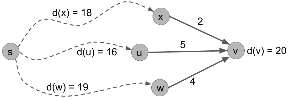
For vertex v, we can check the two points of Fact 1 in the following table. We see that the distance to v is d(v) = 20, which is the minimum over these options.
| d(x) = 18 | wt(x,v) = 2 | d(x) + wt(x,v) = 20 |
| d(u) = 16 | wt(x,v) = 5 | d(x) + wt(x,v) = 21 |
| d(x) = 19 | wt(x,v) = 4 | d(x) + wt(x,v) = 23 |
Dijkstra's
The idea of Dijkstra's algorithm is similar to a modified breadth-first search. We will process vertices in order of their distance from the source. For each vertex, we will set the distances of its neighbors. However, instead of locking in the distance the first time, we will update the distance using the idea of the fact.
The other change is that we need a fancier data structure, which we call a priority queue. In a priority queue, every object in the queue has a value. We always pop the object with the smallest value. Here are the operations; we'll discuss the time complexity later.
Priority Queue:
| Operation | Meaning |
|---|---|
| insert$(u, d)$ | insert object $u$ with value $d$ |
| update$(u, d)$ | update the value of $u$ to be $d$ |
| pop_smallest() | remove and return the object with smallest value |
| size() | return the number of objects in the queue |
Now, we can give Dijkstra's algorithm.
// Algorithm 6: Dijkstra's
1  dijkstra(G, s):
2      // G is a weighted graph with weights w(u,v)
3      let Q = new Priority_Queue
4      for all vertices u:
5          let dist[u] = infinity
6          Q.insert(u, infinity)
7      set dist[s] = 0
8      Q.update(s, 0)
9      while Q.size() > 0:
10         let u = Q.pop_smallest()
11         for each neighbor v of u:
12             set dist[v] = min(dist[v], dist[u] + w(u,v))
13             Q.update(v, dist[v])
14     return dist
As we mentioned, there are two main changes from BFS. The first is to use a priority queue so that we always pop the remaining vertex with minimum distance. The second is that when we process u, we update the distances of all its neighbors v. If dist[v] is currently larger than the distance available by going to u and then hopping to v, we update it.
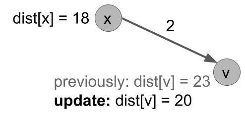
Figure: line 11 of dijkstra(G,s).
As usual with algorithms, the best way to understand it is to execute it by hand on some examples.
Given the below graph, simulate the execution of Dijkstra's algorithm starting from u. Report, at the beginning of each iteration of the while loop, the state of the priority queue and the distance table, and which vertex is popped from the queue.
Example solution.
| Round | dist[u] | dist[v] | dist[w] | dist[x] | dist[y] | queue | vertex popped |
|---|---|---|---|---|---|---|---|
| 1 | 0 | $\infty$ | $\infty$ | $\infty$ | $\infty$ | u, v, w, x, y | u |
| 2 | 0 | 3 | 7 | $\infty$ | $\infty$ | v, w, x, y | v |
| 3 | 0 | 3 | 7 | 5 | $\infty$ | x, w, y | x |
| 4 | 0 | 3 | 7 | 5 | 14 | w, y | w |
| 5 | 0 | 3 | 7 | 5 | 14 | y | y |
| 6 | 0 | 3 | 7 | 5 | 14 | $\quad$ | |
Reconstructing the actual paths
Just as with BFS, the initial version of Dijkstra presented only returns the length of the shortest path, not the path itself. But just as with BFS, it is pretty straightforward to modify the algorithm in the same way: we maintain a prev array, where prev[v] represents the previous vertex for $v$ along the shortest path from $s$. Here is how we update the algorithm, in lines 7 and 15-16.
// Algorithm 7: Dijkstra's with Path Pointers
1  dijkstra(G, s):
2      // G is a weighted graph with weights w(u,v)
3      let Q = new Priority_Queue
4      for all vertices u:
5          let dist[u] = infinity
6          Q.insert(u, infinity)
7          let prev[u] = null
8      set dist[s] = 0
9      Q.update(s, 0)
10     while Q.size() > 0:
11         let u = Q.pop_smallest()
12         for each neighbor v of u:
13             set dist[v] = min(dist[v], dist[u] + w(u,v))
14             Q.update(v, dist[v])
15             if dist[v] == dist[u] + w(u,v):
16                 set prev[v] = u
17     return dist, prev
In particular, in lines 15-16, if the current shortest path to v is indeed from u, then we set prev[v] = u. Given these changes, reconstructing a shortest path can be done with the same algorithm get_path(s, t, prev), from BFS.
Correctness
For graphs with positive edge weights, Dijkstra's algorithm correctly solves the single-source shortest paths problem.
Let us number the vertices in order that the algorithm pops them from the queue: $s=v_1,v_2,v_3,\dots,v_n$.
We prove by induction on $k=1,\dots,n$ that, when we pop $v_k$, its distance is set correctly: dist[v_k] $= d(v_k)$. We note that distances start at $\infty$ and only decrease, and cannot fall below the true distances because every update corresponds to the distance of a path to $v_k$. So if dist[v] $= d(v)$ at any point, the equality holds true forever.
Base case: $k=1$, i.e. the case of $s$. When we pop $s$, we correctly have dist[s] = 0.
Inductive case: Suppose that $v_1,\dots,v_k$ had their distances set correctly when popped. We first note that for all remaining $v$, we have dist[v] equal to the shortest path of the form $s,\dots,u,v$ where all of $s,\dots,u$ have already been popped. This follows because when each in-neighbor $u$ of $v$ was popped, its distance was set correctly by inductive hypothesis and dist[v] = min(dist[v], dist[u] + wt(u,v)) was called.
Now consider the shortest path that is not of this form. It must be of the form $s,\dots,u,v',\dots,v$ where $s,\dots,u$ have been popped, but $v'$ has not. Because $v$ was the smallest object in the priority queue, we must have dist[v] <= dist[v']. But by the note above, since this path starts $s,\dots,u$, if it is a shortest path, it would have dist[v'] = d(v'). So the distance to $v$ along this path, which is only longer, is longer than dist[v]. So this path is longer. So dist[v] is indeed equal to the shortest distance from $s$.
Running time
First, let's analyze Dijkstra for a generic priority queue. Then, we'll plug in specific implementations of the queue. This time, we'll skip any $O(1)$ time operations and just look at how many times each loop runs.
1  dijkstra(G, s):
2      // G is a weighted graph with weights w(u,v)
3      let Q = new Priority_Queue
4      for all vertices u:                          // n iterations
5          let dist[u] = infinity for all u in V
6          Q.insert(u, infinity)
7      set dist[s] = 0
8      Q.update(s, 0)
9      while Q.size() > 0:                          // at most n iterations
10         let u = Q.pop_smallest()
11         for each neighbor v of u:                // at most O(n + m) iterations total
12             let dist[v] = min(dist[v], dist[u] + w(u,v))
13             Q.update(v, dist[v])
14     return dist
The time complexity is therefore $O(n+m)$ plus the time for $O(n)$ calls to Q.insert() and Q.pop_smallest() + O(n + m) calls to Q.update().
A binary tree priority queue
One way to implement a priority queue is with a binary search tree, which keeps its objects sorted by value. In a binary search tree, all operations take $O(\log(n))$ time, where the maximum number of vertices in the tree is $n$.
Binary tree:
| Operation | Time complexity | Meaning |
|---|---|---|
| insert$(u, d)$ | $O(\log n)$ | insert object $u$ with value $d$ |
| update$(u, d)$ | $O(\log n)$ | update the value of $u$ to be $d$ |
| pop_smallest() | $O(\log n)$ | remove and return the object with smallest value |
| size() | $O(1)$ | return the number of objects in the queue |
In this case, our running time is:
$O(n + m + n \log(n) + (n + m)\log(n)) = O((n + m)\log(n))$.
However, there are slightly faster data structures available. The best for Dijkstra's is the Fibonacci heap. It has the amazing property that, over the course of all $n$ insertions and updates, the total time taken is $O(n)$. This is a slightly different statement than saying that the running time is $O(1)$ per update, because there could be a few updates that are slower than that. Hence, we call this kind of guarantee an $O(1)$ "amortized" per operation.
Fibonacci heap:
| Operation | Time complexity | Meaning |
|---|---|---|
| insert$(u, d)$ | $O(1)$ amortized | insert object $u$ with value $d$ |
| update$(u, d)$ | $O(1)$ amortized | update the value of $u$ to be $d$ |
| pop_smallest() | $O(\log n)$ | remove and return the object with smallest value |
| size() | $O(1)$ | return the number of objects in the queue |
With this data structure, our running time is:
$O(n + m + n \log(n) + (n + m) \cdot 1) = O(n \log(n) + m)$.
This is the fastest-known running time for an implementation of Dijkstra's algorithm.