Topic G: Hash Tables and P vs NP
Note: The topics of (1) Hash Tables and (2) P vs. NP are grouped together in this note because it's convenient for class organization, as together they're about the same size as each other topic. However, (1) and (2) are separate topics.
Section 1: Hash Tables
Hash tables are a very useful data structure that use randomness to achieve good performance.
Objectives: After learning this material, you should be able to:
- Use hash tables as sets, key-value stores, and for similar purposes.
- Analyze how hash tables with $m$ bins and $n$ items perform under perfect hashing, ideal (random) hashing, and worst-case hashing.
- Explain the birthday paradox.
A hash table as a data structure
Data structures store and retrieve information. A data structure can be broken down into:
- An interface: what operations does it support?
- An implementation: how do we achieve those operations, and what is the time and space complexity of each?
First, let's think of a hash table as a Set. It will support these operations:
| Operation | Average-case time | Worst-case time | Description |
|---|---|---|---|
| Store(x) | $O(1)$ | $O(n)$ | Add x to the set |
| Get(x) | $O(1)$ | $O(n)$ | Check if x is in the set |
| Remove(x) | $O(1)$ | $O(n)$ | Delete x from the set |
We will discuss the difference between average-case and worst-case time soon.
It is pretty straightforward to modify such a structure to store key-value pairs; such a data structure is often called a table, a dictionary, or a map. If we want to store a key $k$ associated to a value $v$, then we simply treat $k$ as we did $x$ above, and when we go to store it in the data structure, we also store $v$ along with it. Then, when we want to look up $k$, we can find it and also retrieve $v$.
| Operation | Average-case time | Worst-case time | Description |
|---|---|---|---|
| Store(k,v) | $O(1)$ | $O(n)$ | Store key-value pair $k,v$ |
| Get(k) | $O(1)$ | $O(n)$ | Retrieve value $v$ for key $k$, if any |
| Remove(k) | $O(1)$ | $O(n)$ | Delete $k$ and its value |
One can also use a binary tree or other data structures to implement these operations, but not as quickly (in the average case).
An example use case would be counting the number of times each word appears in a document:
// Algorithm 1: Counting words
1 count_words(document):
2     hash_table = new hash table
3     for each word in document:
4         previous_count = hash_table.Get(word)   // or zero if not yet stored
5         new_count = previous_count + 1
6         hash_table.Store(word, new_count)
Implementing hash tables
In general, we will implement a hash table by using an array to store the items. If we have $n$ items, we would like to have an array of length $m=n$, so that there is one slot per item.
To store the items, we will choose in advance a hash function that assigns each item a location in the array.
Given a universe $U$ of items and an array length $m$, a hash function is a function $h: U \to \{1,\dots,m\}$ that assigns each item a location in the array.
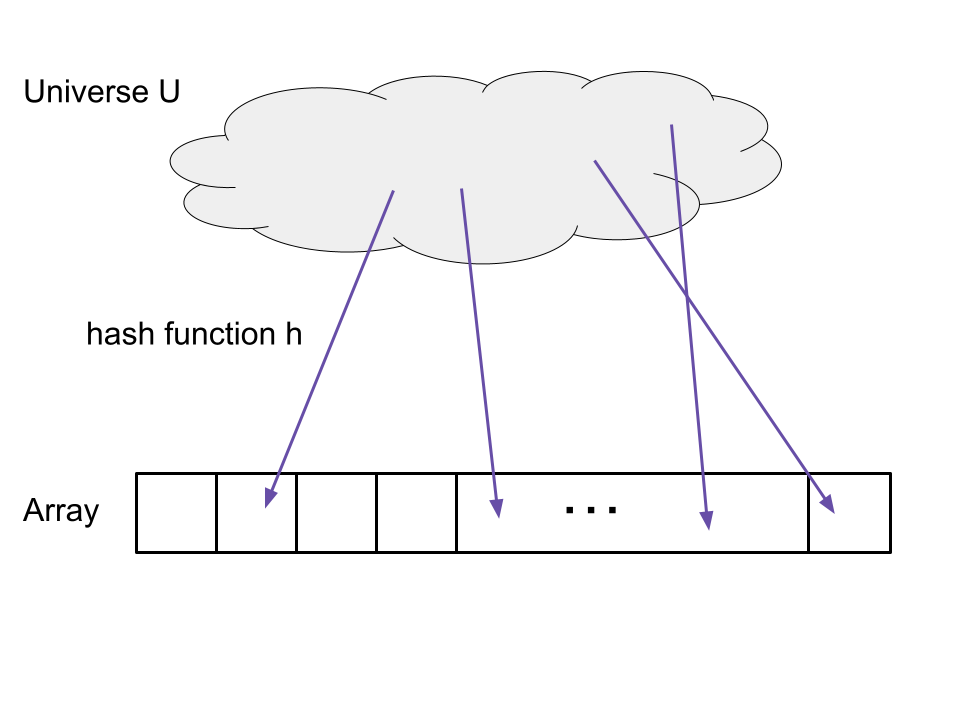
However, the problem is that usually, there is a large "universe" of items that might arrive, much larger than $n$. For example, we may be storing 64-bit integers in a set. In this case, there are $2^{64}$ possible integers that might arrive. Even if only a small number of them do, we don't know in advance which ones.
Suppose we are hashing 64-bit integers to $\{0,\dots,1023\}$. We will use a naive hash function, $h(x) = x % 1024, where % is the "modulo" operator.
Part a. Give a set of $1024$ integers that are "perfectly hashed": each one goes to a different location. Briefly explain.
Part b. Give a set of $1024$ integers that are hashed in the worst way: they all go to the same location. Briefly explain.
Sample solution
Part a. For example, we can take $\{0,1,\dots,1023\}$. Each nubmer is hashed to itself.
Part b. For example, $\{1, 1025, 2049, \dots\}$, that is, the numbers of the form $1024k + 1$ for $k = 0, \dots, 1023$. All of these are hashed to slot 1.
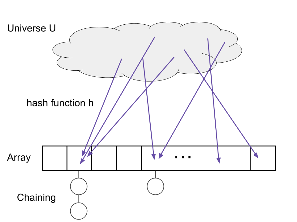
Collisions and chaining
If two items are hashed to the same location, we call this a collision. Every hash table needs a strategy to handle collisions. We will focus on a straightforward strategy called chaining. In chaining, we simply make a list (such as a linked list) for each array location. If multiple items arrive, we add them to the list for that location.
To summarize, the hash table is implemented as follows. Before starting, we pick a hash function h. We will discuss the choice of h later.
Store(x):
- Let j = h(x).
- If there is no item at location j, put x there.
- If there are already items there, add x to the linked list for location j.
Get(x):
- Let j = h(x).
- If there is no item at location j, return None.
- If there is one or more items, look through the linked list for x and return whether you found it.
Remove(x):
- Follow the instructions for Get(x), but if you find x, delete it from the list.
Analysis of hash tables
Suppose we will Store() $n$ items total in a hash table with array length $n$. Then, we will make $n$ calls to Get(). What will be the total time complexity?
We will assume that all of our hash functions run in constant time, $O(1)$, per call.
In the best case, each item is hashed to a different location. Because all of the lists are of length $1$, all of the store and retrieve operations run in constant time. Therefore, the total time is $O(n)$, and each Store() and Get() command runs in $O(1)$ time.
In the worst case, all of the items are hashed to the same location. The time for all of the Store and Get commands is $O(1 + 2 + \cdots + n) = O(n^2)$. Therefore, on average, each Store() and each Get() command runs in $O(n)$ time.
Now, let's consider the average case. To do so, we have to see what hash function we will actually use. We will use randomness to try to "spread out" the hash function's outputs. For analysis, we'll make this assumption.
An ideal hash function is one where each item's location is chosen uniformly at random and independently from $\{1,\dots,m\}$.
Assuming an ideal hash function, each bin has on average one element. Therefore in the average case, each Store() command and each Get() command use O(1) operations. (To be more formal, one can show that the sum over all $n$ Store() and Get() commands is $O(n)$, which gives $O(1)$ per command average-case.)
Using an ideal hash function is modeled by the "balls in bins" problem where we throw $n$ balls (these are the items being hashed) into $m$ bins (the array locations), where each ball lands in a independent, uniformly randomly chosen bin.
Suppose we throw $n$ balls into $n$ bins, i.e. we hash $n$ items into $n$ array slots using an ideal hash function. What is the probability that bin number 1 is empty (has no items)?
Solution.
Each ball misses bin 1 with probability $1 - \frac{1}{n}$. Since they're independent, the probability they all miss is $\prod_{j=1}^n (1 - \frac{1}{n}) = (1 - \frac{1}{n})^n \to \frac{1}{e}$ as $n \to \infty$. So the probability is about $\frac{1}{e} \approx 0.3678$.
To recap, we hope to have a hash function that is as close to "ideal" as possible. In practice, there are many hash functions, and they often do have a randomly chosen component. They often work by using arithmetic operations on the bits of the input in order to "scramble" them and produce a randomly-distributed output.
Another implementation note is that, often, we don't know in advance how many items we'll store in the hash table. This can be addressed by starting with a small table and doubling the size of the table once the number of items grows large enough, reassigning all items to the new array slots. We repeat as needed.
Birthday paradox
When analyzing hash tables, one question is how many collisions will occur and when they will occur. Let's start by asking when the first collision will occur. How many balls do we need to throw into $n$ bins before we expect that two balls have landed in the same bin?
If we throw $k$ balls into $n$ bins, the expected number of collisions is ${k \choose 2} \frac{1}{n} = \frac{k(k-1)}{2n}$.
Consider any pair of balls. What is the probability they land in the same bin? The answer is $\frac{1}{n}$: the first ball lands in some bin, and the second ball has a $\frac{1}{n}$ chance of landing in that bin.
But now the expected number of collisions is just the sum, over all pairs of balls, of the probability that pair collides. There are ${k \choose 2} = \frac{k(k-1)}{2}$ pairs of balls, so the answer is ${k \choose 2}\frac{1}{n}$.
For $k \approx \sqrt{2n}$, after throwing $k$ balls, there is in expectation one collision.
This result is surprising because $\sqrt{2n}$ is much less than $n$; we probably get a collision very quickly! An example is the "birthday paradox". There are about 365 days in a year. If we pretend that each person's birthday is chosen independently and uniformly at random, then how many people do we need in a room before we expect that some pair share a birthday? The answer is only about $27 = \sqrt{2 \cdot 365}$.
This result implies that we need a strategy for handling collisions even when the number of items is much smaller than the size of the array.
Section 2: P and NP
We now switch gears to discuss the complexity classes P and NP.
Objectives: After learning this material, you should be able to:
- Define P.
- Define NP using the verifier definition.
- List common problems in P and NP.
- Prove that a problem is in NP by giving a verifier.
Computational complexity and P
Throughout class, we have asked: how efficiently can you solve a problem? In particular, we often want to know the fastest runtime of any algorithm for a problem such as shortest paths or minimum spanning tree.
Given that, we can also start to classify problems themselves as "easy" (they have a fast algorithm) and "hard" (they have no fast algorithm). We call such classes complexity classes.
More precisely, we'll look at a very permissive definition of easy: running in polynomial time, i.e. running time $O(n^k)$ for some constant $k$. Almost all of the problems we've seen in this class fall into this definition, but we'll see that some care is needed. We'll also need a universal way to measure running time that works for all problems, whether they're on graphs, integers, lists, or any other type of input. We'll do so by measuring the input size in terms of the number of bits needed to write the input down.
An algorithm is a polynomial-time algorithm if there exists a constant $k$ such that, when the input is represented using at most $n$ bits, the running time of the algorithm is at most $O(n^k)$.
Finally, we'll make things simpler by focusing on decision problems.
A decision problem is a problem where the answer is either yes or no.
Many problems can be converted into decision problems. For example, the shortest paths problem can be re-framed as a decision problem: is there any path of length at most $d$? If we can solve shortest paths in polynomial time, then we can solve the decision problem in polynomial time. And conversely, if we had some polynomial-time algorithm for the decision problem, we could use it to solve the original shortest-paths problem by binary search on $d$.
The complexity class $\mathsf{P}$ consists of all decision problems that have a polynomial-time algorithm.
We tend to think of $\mathsf{P}$ as problems that are "easy", or at least "tractable".
NP
Now we will look at a broader class of problems. Informally, NP will be the problems where we can "check" or "verify" a yes-answer in polynomial time. An example is the Hamiltonian path problem: given a directed graph, does there exist a path that visits every vertex exactly once? If the answer is yes, then we can ask for such a path and check that it does indeed vist every vertex once. This is easy to check, if we have the path. (In this case, the path itself is called the "witness" that the answer is yes for this given graph.) But it turns out that we don't know of an efficient (i.e. polynomial-time) algorithm to find such a path.
{Verifier} A verifier for a decision problem is an algorithm that satisfies the following properties.
- The verifier takes as input a pair $(I,W)$ where $I$ is an instance of the decision problem and $W$ is the "witness".
- The verifier outputs either "accept" or "reject".
- The size of the witness satisfies
length(W) <= p(length(I))where $p$ is some polynomial. - If $I$ is a "yes" instance of the decision problem, then there exists at least one witness $W$ such that the algorithm accepts $(I,W)$. ("Completeness")
- If $I$ is a "no" instance of the decision problem, there for any witness $W$, the algorithm rejects $(I,W)$. ("Soundness")
As mentioned, the Hamiltonian Path decision problem is whether a directed graph has a path that visits every vertex exactly once. It has the following verifier:
- The witness string is a list of $n$ of the vertices of the graph.
- Given $(I,W)$, the verifier checks if $W$ is a valid path in the graph and if it contains every vertex exactly once.
- If so, the verifier accepts, otherwise it rejects.
We can see that if there really does exist a Hamiltonian path $v_1,\dots,v_n$, then for witness $W = (v_1,\dots,v_n)$, the verifier will accept. On the other hand, suppose there doesn't exist any Hamiltonian path. In other words, the answer to the problem is "no". Then no matter what witness $W$ is provided, the verifier will always reject, because no list of $n$ vertices can be a valid path that contains every vertex once. So Hamiltonian path has a verifier.
The knapsack decision problem is: given a list of objects with weights and values, and given a knapsack size $W$ and value goal $V$, does there exist a subset of the items with total weight at most $W$ and total value at least $V$? A verifier is the following:
- The witness string is a subset of the objects. (This is polynomially-sized, since it is a list of at most $n$ numbers.)
- Given $(I,W)$, the verifier adds up the values and weights of the objects.
- If the total weight is at most $W$ and the total value is at least $V$, it accepts. Otherwise, it rejects.
If there really does exist such a subset of items, then that subset is a witness that will cause the verifier to reject. On the other hand, if no such subset exists, then the verifier will reject no matter what witness it is given. This follows because any subset will either have too much weight or not enough value. So knapsack has a verifier.
We can now define the complexity class NP.
The complexity class $\mathsf{NP}$ consists of all decision problems that have a polynomial-time verifier.
We can check that our verifiers for Hamiltonian Path and Knapsack, above, both run in polynomial time. Therefore, both of these problems are in NP.
The Hamiltonian Cycle problem is: given a directed graph $G$, does there exists a cycle that visits every vertex exactly once, except the start and end vertices? Prove that the Hamiltonian Cycle problem is in NP.
Example solution.
The witness is the cycle that visits every vertex exactly once. The verifier, given the graph $G$ and a witness string interpreted as a list of vertices, checks that each vertex is in the list once (except the start and end vertex) and checks that the list of vertices is actually a cycle in the graph. If all of these checks pass, it accepts.
This verifier runs in polynomial time, as this is only a linear number of checks (with an adjacency matrix; at most quadratic with an adjacency list). It accepts if and only if the witness is a Hamiltonian Cycle, by definition.
Comparing P and NP
First, we should note that every problem in P is also in NP.
$\mathsf{P} \subseteq \mathsf{NP}$. That is, any problem that has a polynomial-time algorithm also has a polynomial-time verifier.
Suppose a problem has a polynomial-time algorithm $M$. Then the verifier is the following: Given $(I,W)$ where $I$ is an instance of the problem and $W$ is a witness, we ignore the witness and just run the algorithm $M$ on the input $I$. If $M$ outputs "yes", we accept. If it outputs "no", we reject. This verifier runs in polynomial time. It satisfies completeness because for any yes instance $I$, regardless of what witness we use, the verifier accepts. It satisfies soundness because for any no instance $I$, regardless of what witness we use, the verifier rejects.
The largest open problem in Computer Science is whether P and NP are actually the same, i.e. whether P = NP.
Does $\mathsf{P}$ equal $\mathsf{NP}$, or is $\mathsf{NP}$ a strictly larger set? That is, do there exist problems that have a polynomial-time verifier, but have no polynomial-time algorithm?
It's worth mentioning that every problem in $\mathsf{NP}$ can be solved by a brute-force search of the following form:
- Given an instance $I$, iterate through all possible witness strings $W$.
- For each $W$, run the verifier to check if it accepts $(I,W)$. If so, return "yes".
- If the verifier never accepted, then return "no".
However, this takes $\text{poly}(n) 2^{\text{poly}(n)}$ time on inputs of length $n$. The question of P = NP is the question of whether problems that admit this type of brute-force search can always be sped up to polynomial time.
Section 3: NP-Completeness
Finally, we will look at an amazing method to show that some problems are "at least as hard" as others: NP-Completeness
Objectives: After learning this material, you should be able to:
- Define NP-Complete.
- Name some common NP-complete problems
- Prove that a problem is NP-complete using a reduction.
NP-Completeness
Amazingly, there are problems in NP that are "at least as hard" as any other problem in NP. Such problems are called "NP-complete". To define NP-completeness, we will consider reductions, i.e. ways to transform some Problem A into another Problem B. If Problem B is easy to solve, this would imply that A is easy to solve too (by transforming it to B). We will find types of "Problem B" that every problem in NP can be reduced to.
A mapping reduction from decision problem A to decision problem B is an algorithm that, given an instance $I$ of problem A, produces an instance $I'$ of problem B such that $I$ is a "yes" if and only if $I'$ is a yes. It is a polynomial-time mapping reduction if the algorithm runs in polynomial time in the size of its input $I$.
We can now make an amazing definition: NP-Complete. A problem B is NP-Complete if every other NP problem reduces to it.
A decision problem B is NP-Complete if it is in NP and, for every decision problem A in NP, there exists a polynomial-time mapping reduction from A to B.
Here is one reason NP-Completeness is important: if we have a single NP-Complete problem, and we can solve it efficiently, then we can solve every problem in NP efficiently.
If a decision problem B is NP-Complete and if we have a polynomial-time algorithm for B, then P=NP.
Let A be any problem in NP. Because B is NP-complete, there is a polynomial-time mapping reduction $M$ from A to B. Here is a polynomial-time algorithm for A:
- Given an input $I$ for A, use $M$ to produce an input $I'$ for B. Notice that, since M runs in polynomial time, the size of $I'$ is at most $|I'| \leq p(|I|)$ for some polynomial $p$, where $|I|$ is the size of input $I$.
- Run the polynomial-time algorithm for B on $I'$. This takes time $q(|I'|)$, where $q$ is some polynomial. Return the answer.
This algorithm is correct by definition of mapping reduction. It also runs in polynomial time: The running time of $M$ is polynomial in $|I|$, and the running time of the algorithm for B is at most $q(p(|I|))$, where $q$ and $p$ are polynomials. The composition of two polynomials is still a polynomial.
For an example of the $p$ and $q$ used in the proof, imagine that our reduction takes an instance $I$ of length $n$ and produces an instance $I'$ of length $n^2$. And suppose that the algorithm for B runs in time $O(m^3)$ on inputs of length $m$. Then the total running time is $O((n^2)^3) = O(n^6)$.
A first NP-Complete problem
It's not obvious whether there are any NP-Complete problems at all, but there are. Here is our first one: Satisfiability, or SAT for short.
The Satisfiability (SAT) problem is:
- Input: a boolean formula on $n$ variables $x_1,\dots,x_n$, i.e. a combination of logical AND, OR, NOT, and parenthetical groupings of variables.
- Output: "yes" if there exists an assignment of True or False to each variable such that the formula overall evaluates to True; "no" if no such assignment exists.
SAT is in NP.
The witness string is the assignment of True/False to the variables $x_1,\dots,x_n$. The verifier simply plugs the variables into the formula and evaluates it; if True, it accepts, otherwise it rejects.
SAT is NP-Complete.
We already showed that SAT is in NP. We now must show that every problem A in NP has a polynomial-time mapping reduction to SAT.
Let A be a decision problem in NP with a verifier $V$. Here is our mapping reduction. First, we will represent the memory and variables used by $V$ in binary. On input $I$ of size $n$, $V$ uses at most $p(n)$ total bits of memory over the whole course of its operation, for some polynomial $p$, including the input variables. Furthermore, it takes at most $q(n)$ total steps. We will have a new variable $x_{i,j}$ representing memory slot $i$ at time step $j$, where True represents that the bit is set to 1 at that time.
For each possible step $i = 1,2,\dots$ of $V$, we can write down a Boolean formula $f_i$ that evaluates to True if and only if that step was completed correctly. For example, if step $i$ is represented as $z = z + 1$, then the formula would involve the bits of $v$ at step $i-1$ and step $i$ and would evaluate to True if the addition was carried out correctly. (Checking this claim formally would take a lot more detail, but we will skip it here.) We also make a Boolean formula $f_{accept}$ that evalutes to True if and only if the verifier accepts based on its memory state at the last step.
Now, our mapping reduction works as follows. Given an instance $I$ of problem A, we construct the Boolean formula $f_0 \text{ AND } f_1 \text{ AND } \cdots \text{ AND } f_{accept}$. Here $f_0$ is a formula that says the memory of $V$ is correctly initialized to the instance $I$ and that the rest of the memory, except for $W$, is correctly initialized. We let the witness input $W$ remain unconstrained.
The mapping reduction runs in polynomial time because each $f_i$ can be constructed in polynomial time, and there are polynomially many of them. Further, it is correct because it returns a satisfiable formula if and only if there exists a setting of the witness $W$, and a setting of the state variables at each time step, such that the verifier runs as it is supposed to and accepts. If there is no such witness $W$, the formula is not satisfiable because any initial setting of $W$ and setting of the state variables will either not represent a valid operation of $V$, or will result in $V$ rejecting.
More NP-Complete problems
Knowing about NP-Completeness is very important in practice, because many problems turn out to be NP-Complete. If you run into an NP-Complete problem, you know that it has no known polynomial-time algorithm. Therefore, you will need to think about how to approach it: maybe you can try an approximately-correct algorithm, a heuristic, or (if your problem is not too large) turn to algorithms out there tailored for solving NP-Complete problems as fast as possible.
What other problems are NP-Complete besides SAT? It turns out that now that we have one NP-Complete problem, we can have many more by a more simple approach.
If A is NP-Complete, and B is in NP, and A reduces to B with a polynomial-time mapping reduction, then B is NP-Complete too.
For any problem X in NP, we can first take a polynomial-time mapping reduction from an instance $I$ to an instance $I'$ of A, then another reduction to an instance $I''$ of B. Since each reduction runs in polynomial time, this is a polynomial-time mapping reduction from X to B.
To prove another problem is NP-Complete, we just have to show that SAT can be reduced to it. Here are some of the many known NP-Complete problems:
- Hamiltonian Path, defined above.
- Clique problem: given an undirected graph $G$ and integer $k$, does there exist a subset of $k$ vertices that are all pairwise neighbors with each other?
- Knapsack problem, decision problem version: given an instance and a threshold $t$, does there exist a set of items that fit in the knapsack with total value at least $t$?
Knapsack is an interesting case. Recall that we have a dynamic programming algorithm for knapsack that is better than the brute-force approach. However, the algorithm runs in time $O(nW)$ where $n$ is the number of items and $W$ is the weight limit of the knapsack. If we consider the number of bits in the input, it only takes $\log(W)$ bits to write down $W$, so the running time is actually exponential in the size of the input. However, this does show that NP-Complete problems can have better algorithms than pure brute-force search.
Proving a problem is NP-Complete
To prove a decision problem is NP-complete, we have to remember two steps:
- Prove the problem is in NP.
- Prove that an NP-Complete problem reduces to it.
The Hamiltonian Cycle problem is, given a directed graph, to find a cycle that visits every vertex (except the start and end vertex) exactly once. Prove that Hamiltonian Cycle is NP-Complete.
Hint: reduce from Hamiltonian Path.
Sample Solution.
First, we prove the problem is in NP. The witness will be the cycle referenced in the problem. The verifier, given a graph and a list of vertices, checks that the list contains every vertex once except the start and end vertex, which equal each other, and that it is a valid cycle in the graph (i.e. follows existing edges).
Next, we reduce from Hamiltonian Path to Hamiltonian Cycle. Given an instance of Hamiltonian Path, we add a new vertex $w$ to the graph and connect it both to and from every existing vertex. If the previous graph had a Hamiltonian Path, then the new graph has a Hamiltonian Cycle by beginning at $w$, following the Path, and ending at $w$. Conversely, suppose the new graph has a Hamiltonian Cycle. It must contain $w$. By rearranging, we can put $w$ first and last in the Hamiltonian Cycle, i.e. $w, v_1,\dots,v_n,w$. Then the list $v_1,\dots,v_n$ is a path that touches every vertex besides $w$, so it is a Hamiltonian Path in the original graph.