Topic A: Big-O Notation and Complexity
Section 1: Big-O Notation
This section recalls big-O notation. Throughout the course, we will use big-O to analyze algorithms in terms of time and space complexity.
Objectives. After learning this material, you should be able to:
- Recall the formal definition of big-O notation, $f = O(g)$.
- Prove that $f = O(g)$ using a $C,N$ proof.
- Prove that $f = O(g)$ using a limit proof.
- Recall the definitions of big-Omega $\Omega(g)$, big-Theta $\Theta(g)$, little-o $o(g)$, and little-omega $\omega(g)$.
- Sort functions by asymptotic growth rate, from least to highest.
- Given two functions $f,g$, state which of the following are true or false: $f = O(g)$, $f = \Omega(g)$, $f = \Theta(g)$, $f = o(g)$, $f = \omega(g)$.
Motivation and Intuition
We often want to compare algorithms to see which is faster or uses less memory. But that depends on details: the hardware they're running on, the particular inputs, and more. So we'll step back and get a rough sense of an algorithm's performance by bounding its asymptotic performance as the inputs get larger and larger. We will discuss this in detail next chapter, but for now, just know that big-O will be our tool to get rough estimates that don't depend on details such as hardware performance.
Important: big-O applies to any functions, not just runtime or space usage. We will consider the big-O properties of any function $f: \mathbb{R} \to \mathbb{R}$, although we will often have that $f(n)$ is the runtime of an algorithm on inputs of size $n$ (discussed soon).
With big-O, we will focus on the "asymptotic growth rate" of functions as we zoom out and the functions grow toward infinity.
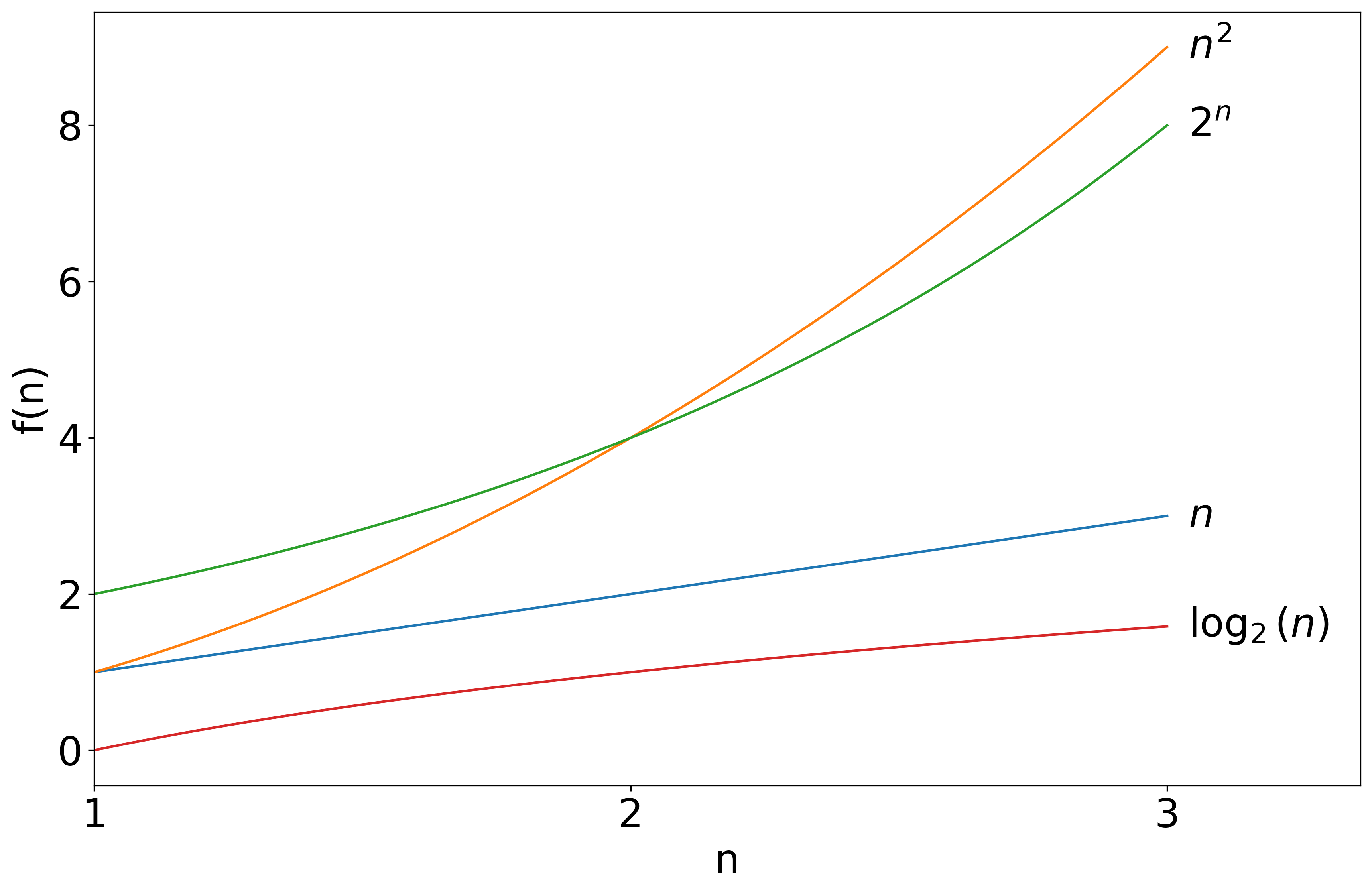
So far, $n^2$ is the largest function, but let's zoom out.
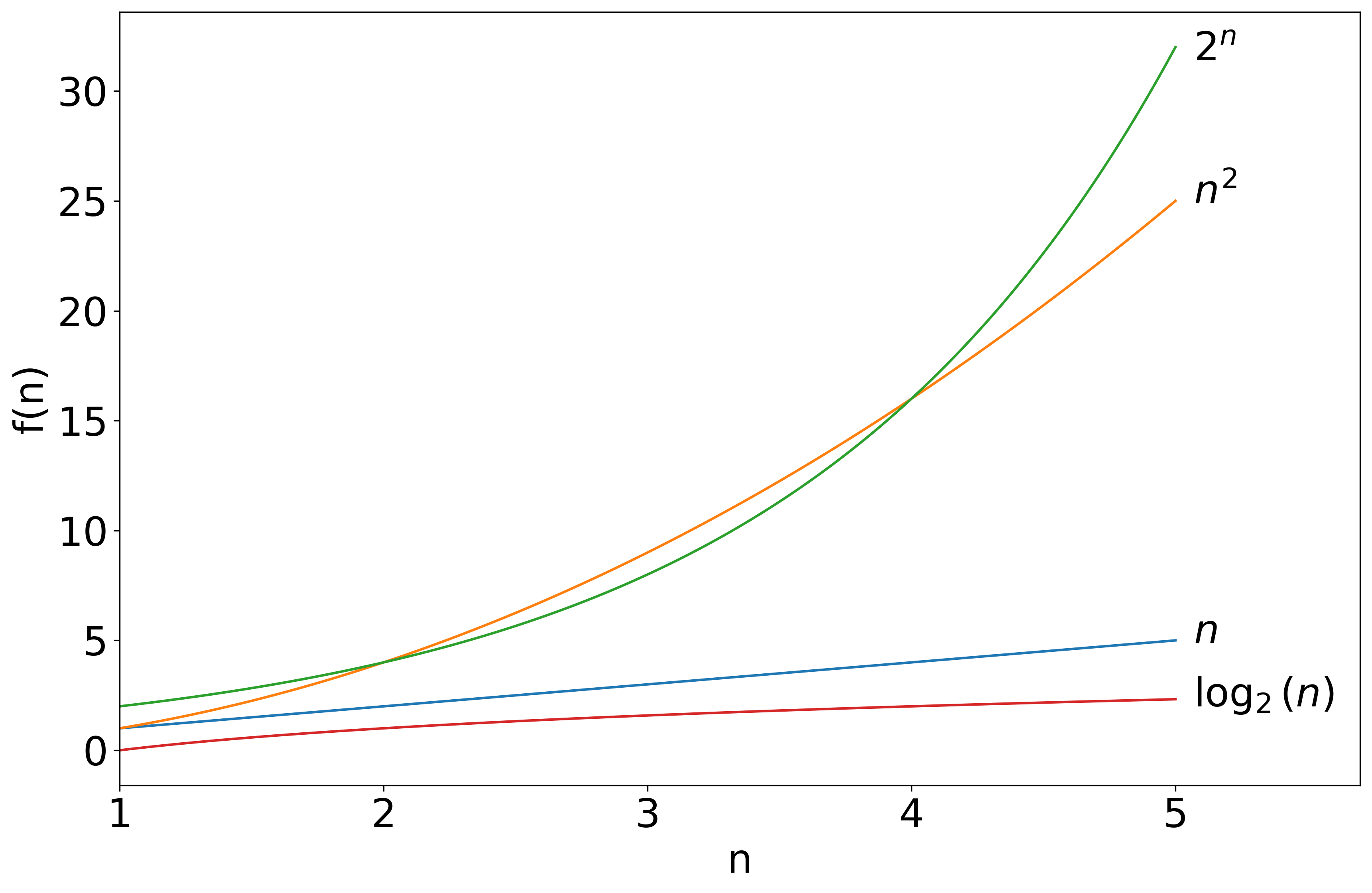
The picture changes as we continue to the right.
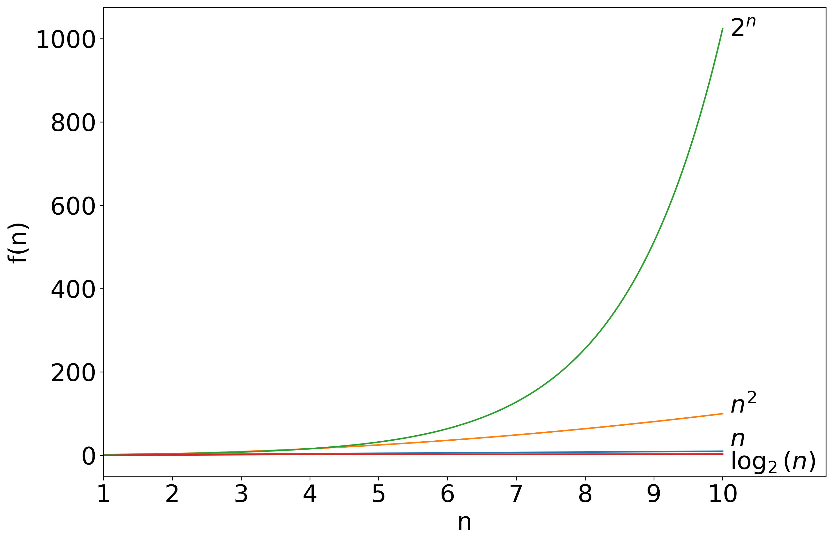
In fact, even if we multiply $n^2$ by a large constant, like 1000, by zooming out, it becomes clear that $2^n$ grows faster. This can also be illustrated with a chart.
| $n$ | $f(n)=n^2$ | $h(n) = 1000n^2$ | $g(n) = 2^n$ |
|---|---|---|---|
| 1 | 1 | 1,000 | 2 |
| 10 | 100 | 100,000 | ~1,000 |
| 20 | 400 | 400,000 | ~1,000,000 |
| 30 | 900 | 900,000 | ~1,000,000,000 |
| 40 | 1,600 | 1,600,000 | ~1,000,000,000,000 |
| 50 | 2,500 | 2,500,000 | ~1,000,000,000,000,000 |
Here, $h(n) = 1000n^2$ begins much larger than $g(n) = 2^n$, but as $n$ increases, the latter quickly becomes much, much larger. We will see that this behavior still occurs if the 1000 in $h(n) = 1000n^2$ is replaced with any constant, however large. On the other hand, in a sense, $f(n) = n^2$ and $h(n) = 1000n^2$ grow at the same rate: the gap between them remains the same, multiplicatively speaking. We will formalize this idea with big-O.
Formalizing Big-O
Let $f: \mathbb{R} \to \mathbb{R}$ and $g: \mathbb{R} \to \mathbb{R}$. Recall this means that $f$ and $g$ are functions that take in real numbers and output real numbers. Also assume that $f(n) > 0$ and $g(n) > 0$ for all $n$, which will be the case for space and runtime and will make our lives simpler.
Say that $f = O(g)$ if there exist positive numbers $C,N$ such that, for all $n \geq N$, $f(n) \leq C \cdot g(n)$.
In this definition, $N$ is a lower cutoff. We only consider the behavior of $f$ and $g$ for "large" inputs, i.e. $n \geq N$. To understand the constant factor $C$, consider the next example.
Let $f(n) = 5n^2$ and $g(n) = n^2$. Here $f$ is larger than $g$, but only by a constant factor. They grow at the same rate: $f = O(g)$. We can prove this by showing that the definition of big-O holds with $N=1$ and $C=5$. Indeed, for all $n \geq 1$, we have $f(n) \leq 5g(n)$, as required.
Let $f(n) = n^2$ and $g(n) = n^3$. We will prove that $f = O(g)$ with constants $C=1,N=1$. To satisfy the definition, we have to prove that, for all $n \geq 1$, we have $n^2 \leq n^3$. We have $n^2 = 1 \cdot n^2 \leq n \cdot n^2 = n^3$, completing the proof.
To understand these proofs, you can plot $f(n)$, $g(n)$, and $C\cdot g(n)$. Visualizing can also be helpful on the examples below.
Let $f(n) = 10n^2$ and $g(n) = n^3$. We will prove that $f = O(g)$ with constants $C=10,N=1$. We have to prove that, for all $n \geq N$, we have $10n^2 \leq C n^3$. In this case, for all $n \geq 1$ we must prove $10n^2 \leq 10n^3$. This holds because $10n^2 \leq 10n^2 \cdot n$ if $n \geq 1$, so $10n^2 \leq 10n^3$.
We can give an alternate proof of the previous example using different constants. Let us pick $C = 1, N=10$. If $n \geq N$, then $n \geq 10$, so $10n^2 \leq n \cdot n^2 = n^3 = C n^3$. We have proven that $10n^2 \leq 1 \cdot n^3$ for all $n \geq 10$.
As the examples show, there is generally not just one correct choice of $N$ and $C$ that works to prove $f = O(g)$. You can now try on the next example. Remember that you are proving an existence statement about $N$ and $C$, so you get to pick whichever $N$ and $C$ you want to make the proof work.
Let $f(n) = 20n^2$ and $g(n) = 5n^3$. Prove that $f = O(g)$.
Note on writing functions. We will often refer to an expression such as $1000n^2$ as being a function, namely the function that maps $n$ to $1000n^2$. If $f(n) = 4n$ and $g(n) = 1000n^2$, all of these are valid ways of writing the same thing:
- $f(n) = O(g(n))$
- $f = O(g)$
- $f = O(1000n^2)$
- $4n = O(g)$
- $4n = O(1000n^2)$
Coming up with, and writing, proofs
To come up with a big-O proof, you often need to do some scratch work and calculation to find $N$ and $C$. You should first do all the scratch work to figure them out, then write a fresh clean proof using the numbers you have found.
Suppose we are asked to prove that $5n^2 + 3 = O(n^2)$. We can first use a common approach for big-O, which is to upper-bound low-order terms by a higher order. In this case, $3 \leq 3n^2$, so $5n^2 + 3 \leq 5n^2 + 3n^2 = 8n^2$. However, here we need to be careful and notice that our inequality $3 \leq 3n^2$ only holds for $n \geq 1$. So to use it, we will need to choose $N$ at least $1$. Now, we note that we can choose $C = 8$ and we will be done, because $8n^2 = Cn^2$. We have found that $N=1,C=8$ will work for our proof.
Warning: the above scratch work is not a proof! Now that we've done the scratch work, we need to turn it into a good proof.
We choose $C=8,N=1$. For all $n \geq 1$, we have $3 \leq 3n^2$. So in this case, $5n^2 + 3 \leq 5n^2 + 3n^2 = 8n^2 = Cn^2$. This proves $5n^2 + 3 = O(n^2)$.
We call this a "$C,N$" proof that $f = O(g)$. Next we'll see a different type of proof, a "limit" proof.
Calculus proofs
Often, the easiest way to prove a big-O statement is to use the following fact.
If $\lim_{n \to \infty} \frac{f(n)}{g(n)} \leq D$ for some real number $D$, then $f = O(g)$.
Let's show that, for $f(n) = 8n^4$ and $g(n) = n^4$, we have $f = O(g)$. We have $\frac{f(n)}{g(n)} = \frac{8n^4}{n^4} = 8$. So $\lim_{n \to \infty} \frac{f(n)}{g(n)} = 8$, so $f = O(g)$.
Using the proposition in this way is called a "limit proof" of big-O. Limit proofs often use the following:
L'Hopital's Rule: If $f(n) \to \infty$ and $g(n) \to \infty$ as $n \to \infty$, then $\lim_{n \to \infty} \frac{f(n)}{g(n)} = \lim_{n \to \infty} \frac{f'(n)}{g'(n)}$, where $f'$ and $g'$ are the derivatives, assuming the limit exists.
Let's use a limit proof to show that, for $f(n) = 3n^2 + 2$ and $g(n) = n^3$, we have $f = O(g)$. We consider $\lim_{n \to \infty} \frac{f(n)}{g(n)}$. Both the numerator and denominator approach infinity as $n$ grows. We have $f'(n) = 6n$ and $g'(n) = 3n^2$. So by L'Hopital's rule, $\lim_{n \to \infty} \frac{f(n)}{g(n)} = \lim_{n \to \infty} \frac{f'(n)}{g'(n)} = \frac{6n}{3n^2} = \frac{2}{n}$. Since $\lim_{n \to \infty} \frac{2}{n} = 0$, we conclude that $\lim_{n \to \infty} \frac{f(n)}{g(n)} = 0$, which is a constant.
Let's use a limit proof to prove that $n^2 = O(e^n)$. Both functions approach infinity. We remember that $\tfrac{d}{dn} n^2 = 2n$ and $\tfrac{d}{dn} e^n = e^n$. So by L'Hopital's rule, $\lim_{n \to \infty} \frac{n^2}{e^n} = \lim_{n \to \infty} \frac{2n}{e^n}$. Now we use L'Hopital's rule again to get $\lim_{n \to \infty} \frac{2}{e^n} = 0$. Since the limit is zero, we have $n^2 = O(e^n)$.
It's useful to remember that $2^n = e^{a \cdot n}$ for a positive constant $a$. Therefore, using the chain rule, $\tfrac{d}{dn} 2^n = \tfrac{d}{dn} e^{a \cdot n} = a e^{a \cdot n} = a 2^n$. In other words, the derivative of $2^n$ behaves almost like the derivative of $e^n$, except that a positive constant comes out front.
Similarly, we recall that $\frac{d}{dn} \ln(n) = \frac{1}{n}$, and $\log_2(n) = b \ln(n)$ for some positive constant $b$. This means that $\log_2(n) = O(\ln(n))$ and vice versa.
Let's use a limit proof to prove that $\log_2(n) = O(2^n)$. Both functions approach infinity as $n \to \infty$, so we can use L'Hopital's rule. $\lim_{n \to \infty} \tfrac{\log_2(n)}{2^n} = \lim_{n \to \infty}\frac{c (1/n)}{2^n}$ for some constant $c > 0$. Continuing, we get $\lim_{n \to \infty} \frac{c}{n 2^n} = 0$, because the numerator is a constant and the denominator approaches infinity. Since the limit is zero, $\log_2(n) = O(2^n)$.
Comparing growth rates
Here are some of the most common types of functions you will encounter.
- Constant functions: $f(n) = a$ for some real number $a$. All constant functions can be described as $O(1)$.
- Linear functions: $f(n) = a \cdot n$ for some positive constant $a$, such as $f(n) = 4n$. We can abuse terminology and use "linear" to refer to functions of the form $a \cdot n + b$ for some positive constant $a$ and some constant $b$, such as $f(n) = 4n + 2$.
- Quadratic functions: $f(n) = a \cdot n^2$ for some positive $a$.
- Polynomial functions: these are functions of the form $f(n) = a_k n^k + a_{k-1} n^{k-1} + \cdots + a_1 n + a_0$ for some constants $a_0,\dots,a_k$. Examples include $f(n) = 8n^3 - 2n^2 + 4n + 1$ and $f(n) = 5n^{100} + 2n^{33}$. Linear and quadratic functions are examples of polynomials, as are constant functions. In this context, we usually assume $a_k$ is positive so that $f(n) \to \infty$ as $n \to \infty$. We say that the degree of the polynomial is $k$, where $k$ is the highest power.
- More generally, if $f(n) = n^a$ for some positive constant $a$, even if $a$ is not an integer, we abuse terminology and say that $f$ has a polynomial growth rate.
- Logarithmic functions: these are functions of the form $f(n) = \log_2(n)$, or more generally $f(n) = a \cdot \log_2(n)$ for some positive constant $a$. Remember your rules of logarithms! $a \log_2(n) = \log_2(n^a)$.
- Polylogarithmic functions: these are less common, but they are functions of the form $\left(\log_2(n)\right)^k$ for some positive constant $k$, e.g. $(\log_2(n))^2$. Logarithmic functions are polylogarithmic, corresponding to the case $k=1$.
- Exponential functions: these are functions of the form $2^{a \cdot n}$ for positive constant $a > 0$. Sometimes, other functions with $n$ in the exponent, such as $2^{n^2}$, are also referred to as being exponential in $n$.
We always have the following rules of comparison with regard to big-O:
constant $\ll$ polylogarithmic $\ll$ polynomial $\ll$ exponential
where $\ll$ is shorthand for "is big-O of". Furthermore, we can say the following:
If $f(n)$ is a polynomial of degree $k$, then $f = O(n^k)$.
And:
If $k' \geq k$, then $n^k = O(n^{k'})$.
Another useful rule of thumb is that if $a,b > 1$, then $\log_a(n) = O(\log_b(n))$ and vice versa, where $a$ and $b$ are the bases of the logarithms. Because of this, we can be a bit informal and not always specify the bases of our logarithms. In this class, $\log(n)$ will generally mean log base $2$ and $\ln(n)$ will always mean log base $e$. All of these facts can be proven using the $C,N$ definition of big-O (or using calculus, for example).
Suppose we are asked to compare $f(n) = 10 \log(n)$ and $g(n) = 10^n$. Do we have $f = O(g)$, $g = O(f)$, both, or neither?
Solution.
We have $f = O(g)$, but not the other way around. Logarithmic functions grow much slower than exponential functions.
Compare $f(n) = 8n^3 + 2n^2$, $g(n) = 0.1 n^4$, and $h(n) = (\log(n))^{300}$. Order them by asymptotic growth rate from least to highest.
Other functions
There are many functions that do not fall directly into the categories listed above. A common example in computer science is the function $f(n) = n \log(n)$. Comparing the growth rate of such functions may require a little bit of work.
We prove that $n \log(n) = O(n^2)$ using a $C,N$ proof. In this class, you may take as given the fact that $\log(n) \leq n$ for all $n \geq 0$, when the log is base $2$ or $e$. This can be proved directly with calculus. Using this fact, $n \log(n) \leq n \cdot n = n^2$ for all $n \geq 0$. We conclude that, with $N=0$ and $C=1$, the definition of big-O is satisfied.
Other Asymptotic Notation
There are several other pieces of asymptotic notation to remember. We will often use these pieces of notation, although big-O is the most common.
We say $f = \Omega(g)$ if $g = O(f)$.
In other words, big-Omega says that $f$ grows asymptotically at least as fast as $g$. For example, $2^n = \Omega(n)$.
We say $f = \Theta(g)$ if $f = O(g)$ and $g = O(f)$.
In other words, $f$ and $g$ grow asymptotically at the same rate. For example, any two polynomials of the same degree are big-Theta of each other. E.g., take $f(n) = 3n^2 + 200$ and $g(n) = 45n^2 - 30$, then $f = \Theta(g)$. We can prove this by first proving $f = O(g)$, then proving $g = O(f)$.
We say $f = o(g)$ if $\lim_{n \to \infty} \frac{f(n)}{g(n)} = 0$.
In other words, $f$ does not grow as fast as $g$. For example, $n = o(n^2)$. In fact, if $k' > k$, the $n^k = o(n^{k'})$. This is direct to prove from the definition of little $o$.
We say $f = \omega(g)$ if $g = o(f)$.
In other words, $f$ grows "strictly" faster than $g$. Little-omega mirrors little-o in the same way that big-Omega mirrors big-O.
Here is a quick guide, but remember that this comparison to inequality operators is only an analogy.
| Symbol | similar to | English meaning (up to a constant factor) |
| $O(n)$ | $\leq$ | asymptotically at most |
| $o(n)$ | $<$ | asymptotically less; shrinking compared to |
| $\Omega(n)$ | $\geq$ | asymptotically at least |
| $\omega(n)$ | $>$ | asymptotically more; diverging compared to |
| $\Theta(n)$ | $=$ | asymptotically the same |
Based on our previous discussions, we know the following general facts.
- If $f$ is polylogarithmic and $g$ is polynomial, then $f = o(g)$.
- If $f$ is exponential and $g$ is polynomial, then $f = \omega(g)$.
- If $f$ is bounded by a constant and $g(n) \to \infty$, then $f = o(g)$.
You should now be able to answer the following questions.
- Let $f(n) = 2n^2$ and $g(n) = \log(n)$. Which of the following are true and which are false? $f = O(g)$, $f = \Omega(g)$, $f = \Theta(g)$, $f = o(g)$, $f = \omega(g)$.
- Let $f(n) = 8^n$ and $g(n) = n\log(n)$. Which of the following are true and which are false? $f = O(g)$, $f = \Omega(g)$, $f = \Theta(g)$, $f = o(g)$, $f = \omega(g)$.
Closing Comments
One very useful fact is that if $f = O(g)$ and $h = O(g)$ also, then $f + h = O(g)$. We can interpret this as a fact about running times of algorithms: if we have two algorithms with running times $f$ and $h$ respectively, and both of them are $O(g)$, the running first one algorithm and then the other will give an asymptotic running time of $f+h = O(g)$ as well.
Section 2: Analyzing Algorithms
This section introduces the analysis of time and space complexity of algorithms.
Objectives. After learning this material, you should be able to:
- Relate actual code running on hardware to our model of pseudocode used for time and space analysis.
- Use big-O notation to bound the time and space usage of an iterative algorithm.
- Analyze time and space usage of algorithms with nested for loops.
Background
Imagine we want to sort a list of numbers. We have two algorithms. Which is faster? The answer depends on the details, for example:
- What programming language is each written in?
- What hardware is each running on? What is the speed of the processor, the size of the cache, the memory available, and so on?
- What does the problem instance look like? For example, are the numbers already close to being sorted, or in a random order, or arranged in some pattern?
Our goal is a systematic study of algorithm performance that strikes a balance between two goals.
- Our analysis should be relevant to practice, e.g. deciding which algorithm to use.
- Our analysis should be generalizable: it shouldn't only hold for one particular programming language or hardware architecture.
We will introduce a method of analysis that strikes a balance. We will analyze pseudocode that can be translated into most programming languages. The pseudocode's commands will roughly correspond to steps that are taken on any modern CPU. Therefore, the time analysis of the psuedocode will be pretty closely related to the actual running time of an implementation of an algorithm.
Correctness of Pseudocode
First, a quick note on correctness. There are two types of algorithms: correct, and incorrect. But what does it mean for an algorithm to be correct?
We will formalize the problem the algorithm is trying to solve as a mathematically well-defined function from inputs to outputs. The algorithm is correct if, for every possible input, it produces the correct output. We will often prove correctness of our algorithms, and to do so, we must always prove that they always produce the correct outputs.
Analysis of Pseudocode
Throughout the class, we will focus on algorithms written in pseudocode. We will define how much time and space each allowable operation takes. This will allow us to assign a running time and space usage to any algorithm written in pseudocode.
Summing a list of numbers.
// Algorithm 1
1 sum(A):              // A = list of length n
2     let n = len(A)
3     let s = 0
4     for i = 1 to n:
5         s += A[i]
6     return s
We won't worry about specific syntax, such as "let s = 0" versus some other way of initializing a variable, as long as the meaning is clear.
Pseudocode operations
In our pseudocode, we will generally have the following rules and operations. We will assume they take the given number of units of time, called steps, and the given amount of space.
- Variables can be integers, floating-point numbers, booleans, or characters in a string. They can also be objects, such as arrays.
- Declaring a variable or an array. This operation takes $1$ step. Each variable takes $1$ space. An array of $n$ variables takes $n$ space, but the array still only takes one time step to declare. We also assume that appending to an array and expanding it by one spot takes constant time.
- Assigning a new value to a variable. This takes one step and no additional space.
- Reading the value in a variable. This takes one step and no additional space.
- Arithmetic operations such as $+, -, *, /$. These take one step and use no space on their own. Other operations including modulo, exponentiation, and XOR are also generally allowed.
- If, then, else statements. These each take one step and use no additional space on their own.
- For and while loops. These take one step at each control flow location, i.e. the start and end of the loop. (We can think of them as combining an if/then/else statement with goto statements that take one step.) They use no additional space on their own.
- Function calls. Calling a function takes one step and uses one space in addition to the usage of the function itself. We will not generally worry about the space usage, but it is technically important for recursive algorithms.
Let us analyze the time and space usage of Algorithm 1. First, let's look at time, or the number of steps taken to run the algorithm.
// Algorithm 1
1 sum(A):
2     let n = len(A)     // 1 step
3     let s = 0          // 1 step
4     for i = 1 to n:    // 1 step each loop
5         s += A[i]      // 5 steps each loop: read s,i,A[i]; add; store in s
6     return s           // 1 step
Each execution of the loop takes $6$ steps, and the loop executes $n$ times, so the total number of steps taken by lines 3 and 4 is $6n$ steps. Adding the time for lines 2, 3, and 6, we get a running time of $6n+3$.
Now let's look at space usage.
// Algorithm 1
1 sum(A):
2     let n = len(A)     // 1 space
3     let s = 0          // 1 space
4     for i = 1 to n:    // 1 space for i (total)
5         s += A[i]      // no new space
6     return s           // no new space
Summing up the space used gives a total of $3$ space used by the algorithm. We will generally not count the input as part of the space used, although usually, it won't matter because most algorithms use more space than the input.
Note on pseudocode conventions. Pseudocode isn't precisely defined to follow a highly specific format; that's part of the point. We may use slightly different notation and conventions, and you may as well. For example, in Algorithm 1, the array is 1-indexed, meaning that that first element appears at A[1], not A[0]. You may use zero-indexing if you like.
Note on realism. Our estimates here are very rough compared to reality. For example, computers can carry out additions extremely quickly compared to accessing memory storage, but here we treat both as taking the same amount of time. However, this rough approximation still turns out to usefully capture the differences in performance between algorithms much of the time.
Another simplification is that we are not considering parallelism (ability to execute multiple commands at the same time). This model can be extended to analyze parallel algorithms, but we won't do that in this class.
Note on exact runtime. Even in an algorithm as simple as Algorithm 1, it can be a bit unclear exactly how much time and space is used down to the exact number. For example, the for loop includes an implicit branch back to the start, which we did not include in our analysis. Luckily, this won't matter, because we are going to use big-O analysis, which will come out to the same answer regardless of these minor details. That is one of the main points of using big-O. We discuss this next.
Big-O analysis of pseudocode
Given that so many details are implementation-dependent, the running time and space usage we calculate is only approximate. For example, a slightly different analysis of Algorithm 1 could give a running time of $7n+2$ instead of $6n+2$.
Instead of worrying too much about this, we will "lean in" and use big-O to express the time and space usage of our algorithms. Both $7n+2$ and $6n+2$ are $O(n)$, so we say the time complexity of Algorithm 1 is $O(n)$. Similarly, the space usage is $3 = O(1)$, meaning a constant space independent of $n$ (remember that we are not counting the input array in the space usage).
Therefore, instead of worrying about exact constants such as $6n$ versus $7n$, we will worry about the asymptotic growth rate, such as linear time ($O(n)$) versus quadratic time ($O(n^2)$). So our analyses should always follow this approach:
- Analyze the algorithm to produce an expression such as $6n+2$ for the time or space usage.
- Use big-O to give a "simplified" big-O expression, such as $O(n)$.
Simplified expressions should look like simple functions such as $O(n)$, $O(n \log(n))$, $O(n^2)$, etc. They should follow these guidelines:
- Drop leading constants. For example, instead of $O(5n^3)$, write $O(n^3)$, which has the same meaning but is simpler.
- Drop low-order terms from a summation. For example, instead of $O(n^3 + 2n^2)$, write the simpler and equivalent $O(n^3)$.
- Simplify inside expressions where possible. For example, instead of $O(\log(8n^3 + 5))$, write $O(\log(n))$. (Can you prove that $\log(8n^3 + 5) = O(\log(n))$?)
- However, avoid using an asymptotically loose upper bound. It is true that $\log(8n^3 + 5) = O(n^2)$, but $O(n^2)$ is too loose of a bound. The best answer here is $O(\log(n))$.
Worst-case analysis
Algorithm 1 used the same amount of time and space regardless of the input. This is not always the case. Consider the following algorithm.
// Algorithm 2: finding the first nonzero element
1 find_nonzero(A):
2     n = len(A)
3     for i = 1 to n:
4         if A[i] != 0:
5             return A[i]
6     return "none"
What is the time complexity of Algorithm 2?
// Algorithm 2: finding the first nonzero element
1 find_nonzero(A):
2     n = len(A)             // 1 step
3     for i = 1 to n:        // 1 step per loop
4         if A[i] != 0:      // 1 step per loop
5             return A[i]    // 1 step if and when it executes
6     return "none"          // 1 step if and when it executes
We can see that the total time usage is $2k + 2$, where $k$ is the number of loops that execute. But how many is that? It depends on the input array. There is no single correct answer.
To address this, we will typically use a worst-case analysis of the time and space usage of our algorithms. Here, the question is to bound the running time in the worst-case (i.e. slowest) over all possible inputs. Because the worst case is that the loop executes $n$ times, the worst-case running time of the algorithm is $2n+2 = O(n)$.
Unless otherwise specified, in this course, we will always be using a worst-case analysis for both time and space.
Note on input size and parameters. If we say an algorithm has running time of e.g. $O(n)$, we must always ask carefully: what is $n$? In the above context, the input was a list of $n$ numbers. So the time of the algorithm grows linearly in the size of the input. Sometimes, our input will be described by multiple parameters. For example, we may have a matrix with $n$ rows and $m$ columns. Our running time bound may be a function of both $n$ and $m$ in this case.
In computational complexity theory, we often represent the input as a string of bits that encodes the problem, and we care about running time in terms of the number of bits. That will generally not be the case for this class, though.
Examples: Nested Loops
We'll now look at some more complex algorithms involving nested loops.
Counting equal pairs
In this problem, we are given an array A. We must count how many pairs of indices (i,j) there are such that A[i] == A[j].
// Algorithm 3: Counting Equal Pairs
1  count_equal_pairs(A):
2      let n = len(A)
3      let s = 0
4      for i = 1 to n:
5          for j = 1 to n:
6              if A[i] == A[j]:
7                 s += 1
8      return s
Bound the asymptotic time complexity of Algorithm 3. Show your work.
Example solution.
Because of the big-O approach, we will treat constant-time operations as taking one unit of time even if they involve several steps at once, such as reading from memory and comparing. First, we'll write the number of steps each instruction takes.
// Algorithm 3
1  count_equal_pairs(A):
2      let n = len(A)            // 1 step
3      let s = 0                 // 1 step
4      for i = 1 to n:           // 1 step each time executed
5          for j = 1 to n:       // 1 step each time executed
6              if A[i] == A[j]:  // 1 step each time executed
7                 s += 1         // 1 step each time executed
8      return s                  // 1 step
To count how many times each instruction is executed, we first look at the inner for loop, which covers lines 5-7. In the worst case, line 7 is executed every time, so the loop takes 3 steps every iteration. There are n iterations of the loop. So we can write:
// Algorithm 3
1 count_equal_pairs(A):
2     let n = len(A)            // 1 step
3     let s = 0                 // 1 step
4     for i = 1 to n:           // 1 step each time executed
5         // do at most 3n steps
6     return s                  // 1 step
The for loop starting in line 4 also runs n times, and we use $3n+1$ operations each time. This gives a total of $n(3n+1) = 3n^2 + n$ operations coming from that for loop:
// Algorithm 3
1 count_equal_pairs(A):
2     let n = len(A)            // 1 step
3     let s = 0                 // 1 step
4     // do at most 3n^2 + n steps
5     return s                  // 1 step
The total number of steps is $3n^2 + n + 3 = O(n^2)$ steps, so the final answer is $O(n^2)$.
Counting duplicate pairs (without double-counting)
If we consider running Algorithm 3 above on input A = [3, 5, 8, 5], what will the answer be?
It will be 6. The algorithm will find an equal pair every time i==j, i.e. at index 1, 2, 3, and 4. Then, it will find an equal pair when i==2 and j==4, i.e. A[2] == A[4] == 5. Then, it will also find an equal pair when i==4 and j==2. This adds up to 6.
A related task is to count duplicates in the array without double-counting. For the example above, there is one pair of duplicates: indices i==2 and j==4, which both contain the entry 5. To avoid double-counting, we can modify our algorithm as follows.
// Algorithm 4: Counting Duplicates
1  count_duplicates(A):
2      let n = len(A)
3      let s = 0
4      for i = 1 to n-1:
5          for j = i+1 to n:
6              if A[i] == A[j]:
7                  s += 1
8      return s
The difference from Algorithm 3 is that now, the bounds of the for loops are different. Algorithm 3 looped over all pairs (i,j), e.g. (1,1), (1,2), (1,3), (1,4), (2,1), (2,2), (2,3), .... But here, Algorithm 4 only loops over pairs where i < j. This ensures that each pair of indices only gets considered once. For example, (1,2), (1,3), (1,4), (2,3), (2,4),....
Bound the asymptotic runtime of Algorithm 4. Show your work.
Example solution.
Again, we start by noting that each line, on its own, is a constant-time operation.
// Algorithm 4
1  count_duplicates(A):
2      let n = len(A)            // 1 step
3      let s = 0                 // 1 step
4      for i = 1 to n-1:         // 1 step each time
5          for j = i+1 to n:     // 1 step each time
6              if A[i] == A[j]:  // 1 step each time
7                  s += 1        // 1 step each time
8      return s                  // 1 step
Again, we see that the inner loop, lines 5-7, uses 3 steps each time it executes. But how many times does the inner loop execute? It depends on i. When i=1, it executes n-1 times (i.e. from j=2 up to j=n). When i=n-1, it executes 1 time (i.e. from j=n to j=n). In each case, we can say that it executes exactly $n-i$ times.
// Algorithm 4
1 count_duplicates(A):
2     let n = len(A)            // 1 step
3     let s = 0                 // 1 step
4     for i = 1 to n-1:         // 1 step each time
5         // take 3(n-i) steps
6     return s                  // 1 step
Now, we calculate the total time of the outer for loop, which starts on line 4. We need to add up the time taken from each iteration.
Aside (not part of the sample solution). It never hurts to do an example. Let's suppose n=4. Then when i=1, we take 3(4-1) = 9 steps. When i=2, we take 3(4-2) = 6 steps. When i=3, we take 3(4-3) = 3 steps. The total is 9 + 6 + 3 = 18.
To add them up, the expression is $\sum_{i=1}^{n-1} 3(n-i) = 3 \sum_{i=1}^{n-1} (n-i)$. Now, the summation is $(n-1) + (n-2) + \cdots + 2 + 1$, which is the same as $1 + 2 + \cdots + (n-2) + (n-1) = \sum_{i=1}^{n-1} i$. We recall from Discrete Math that the sum of $1$ up to $n-1$ equals $n(n-1)/2$. Therefore, the total number of steps for the loop is
We have reached this stage:
// Algorithm 4
1 count_duplicates(A):
2     let n = len(A)            // 1 step
3     let s = 0                 // 1 step
4     // take (3/2)n^2 - (3/2)n steps
5     return s                  // 1 step
The total number of steps is therefore $\frac{3}{2}n^2 - \frac{3}{2}n + 3 = O(n^2)$ steps.
Comparison with Equal Pairs. Algorithm 4 is certainly faster than Algorithm 3, since its bounds on the for loops are smaller -- sometimes, much smaller. However, we ended up with the same asymptotic bound on the runtime, namely quadratic: $O(n^2)$. In fact, Algorithm 4 takes around half the number of steps of Algorithm 3, but the "half" is a constant factor that does not ultimately affect the big-O runtime bound.
An example with doubling
Now we will consider an example with a "while" loop.
What is the asymptotic runtime of the following algorithm? Show your work. For simplicity, you may suppose that $n$ is a power of two, i.e. $n = 2^m$ for some integer $m$.
// Algorithm 5
1 celebrate(n):
2    k = 1
3    while k <= n:
4       for i = 1 to k:
5          print("hip hip")
6       print("hooray")
7       k *= 2
Example solution.
We first consider the time taken in each line:
1 celebrate(n):
2    k = 1                   // 1
3    while k <= n:           // 1 each outer loop
4       for i = 1 to k:      // 1 each inner loop
5          print("hip hip")  // 1 each inner loop
6       print("hooray")      // 1 each outer loop
7       k *= 2               // 1 each outer loop
The inner loop executes $k$ times and takes 2 steps each time, for a total of $2k$.
The outer loop therefore takes $2k+3$ time steps in each loop as a function of $k$.
We need to add up the total over the outer loops. $k$ starts at 1 and doubles until it reaches $n$, so the time is bounded by
The log is base 2. We got $3(\log(n) + 1)$ because there are $\log(n)+1$ terms in the sum, because the outer while loop executes $\log(n)+1$ times: when $k=1, k=2, k=4, \dots, k=n$. In other words, $k=2^0, 2^1, 2^2, \dots, 2^{\log(n)}$.
Now we recall that $1 + 2 + 4 + 8 + \cdots + n = 2^0 + \cdots + 2^{m} = 2^{m+1}-1$. In this case, $m = \log(n)$, so the sum is $2^{\log(n)+1}-1 = 2 \cdot 2^{\log(n)} - 1 = 2n - 1$. So the running time is
Taking big-O, we get a time complexity of $O(n)$.