Tight Bounds for Gaussian Tails and Hazard Rates
Posted: 2018-03-17.
This post will show how to tightly bound the tail probabilities of the Gaussian distribution from both sides with a closed form.
For example, an upper bound we will show is that if $X$ is Normal(0,1), then for all $x \gt 0$:
\[ \Pr[X \gt x] \leq \frac{1}{\sqrt{2\pi}} \left(\frac{1}{x} - \frac{1}{x^3} + \frac{3}{x^5}\right) e^{-x^2/2} . \]Totally Normal
The "standard" normal distribution $N(0,1)$ has mean zero, variance $1$, and probability density function
\[ \phi(x) := \frac{1}{\sqrt{2\pi}} e^{-x^2/2} . \]It cumulative distribution function is
\begin{align} \Phi(x) & := \Pr[ X \leq x ] \\ & = \int_{-\infty}^x \phi(t) dt . \end{align}The goal is to get good closed-form bounds on $1 - \Phi(x)$ for $x \gt 0$, both upper and lower.
Also, remember that if $Y$ is $N(\mu,\sigma^2)$, then $\Pr[Y \leq y] = \Phi\left(\frac{y-\mu}{\sigma}\right)$ and the density at $y$ is $\frac{1}{\sigma}\phi\left(\frac{y-\mu}{\sigma}\right)$.
Basic Bounds
A starting point would be standard concentration bounds. In particular, Gaussians are subgaussian -- $1$-subgaussian for a Normal(0,1) variable -- so by subgaussian bounds we have \begin{align} \Pr[ X \gt x ] & = 1 - \Phi(x) \\ & \leq e^{-x^2/2} \\ & = \sqrt{2\pi} \phi(x) . \end{align} However, there's a simple, well-known argument that shows we can get better (tighter upper bounds on this tail probabaility. It's worth reviewing carefully, as we will generalize it later. Note that if $f(t) = - e^{-t^2/2}$, then $\frac{df}{dt} = t e^{-t^2/2}$.
Theorem 1. For all $x \gt 0$, $1 - \Phi(x) \leq \frac{1}{x} \phi(x)$.
Proof. \begin{align} 1 - \Phi(x) & = \int_x^{\infty} \phi(t) dt \\ & = \frac{1}{\sqrt{2\pi}} \int_x^{\infty} e^{-t^2/2} dt \\ & \leq \frac{1}{\sqrt{2\pi}} \int_x^{\infty} \frac{t}{x} e^{-t^2/2} dt \\ & = \frac{1}{x} \frac{1}{\sqrt{2\pi}} \int_x^{\infty} t e^{-t^2/2} dt \\ & = \frac{1}{x} \frac{1}{\sqrt{2\pi}} \left[ - e^{-t^2/2} \right]_{x}^{\infty} \\ & = \frac{1}{x} \frac{1}{\sqrt{2\pi}} e^{-x^2/2} \\ & = \frac{1}{x} \phi(x) . \end{align}
Method: Simplest Examples
Now, we can modify this argument by cleverly choosing some factor inside the integral (above, we used $\frac{t}{x}$) so that we can evaluate the integral in closed form. Let's do the simplest upper and lower bound examples, then the general theorem in the next section. First, we'll prove the same bound, but in a different way, which will generalize.
Theorem 1 (again). For all $x \gt 0$, $1 - \Phi(x) \leq \frac{1}{x} \phi(x)$.
Proof. First, note that \begin{align} \frac{d\phi}{dt}\ & = \frac{1}{\sqrt{2\pi}} \frac{d}{dt}e^{-t^2/2} \\ & = \frac{1}{\sqrt{2\pi}} (-t) e^{-t^2/2} \\ & = - t \phi(t) . \end{align} Second, let $f(t) = -\frac{1}{t}\phi(t)$. Note that \begin{align} \frac{df}{dt} & = -\frac{d\phi}{dt} \frac{1}{t} - \phi(t) \frac{d}{dt}\left(\frac{1}{t}\right) \\ & = -\frac{d\phi}{dt} \frac{1}{t} + \phi(t) \frac{1}{t^2} \\ & = \phi(t) \left(1 + \frac{1}{t^2}\right) . \end{align} So \begin{align} 1 - \Phi(x) & = \int_x^{\infty} \phi(t) dt \\ & \leq \int_x^{\infty} \phi(t) \left(1 + \frac{1}{t^2}\right) dt \\ & = \left[f(x)\right]_x^{\infty} \\ & = -f(x) \\ & = \frac{1}{x} \phi(x) . \end{align}
Next, let's do a lower bound that is very close to matching.
Theorem 2. For all $x \gt 0$, $1 - \Phi(x) \geq \left(\frac{1}{x} - \frac{1}{x^3}\right) \phi(x)$.
Proof. Let \[ f(t) = -\left(\frac{1}{t} - \frac{1}{t^3}\right)\phi(t) . \] Note that \begin{align} \frac{df}{dt} & = -\frac{d\phi}{dt} \left(\frac{1}{t} - \frac{1}{t^3}\right) -\phi(t) \left(-\frac{1}{t^2} + \frac{3}{t^4}\right) \\ & = t \phi(t)\left(\frac{1}{t} - \frac{1}{t^3}\right) -\phi(t) \left(-\frac{1}{t^2} + \frac{3}{t^4}\right) \\ & = \phi(t)\left(1 - \frac{1}{t^2} + \frac{1}{t^2} - \frac{3}{t^4}\right) \\ & = \phi(t)\left(1 - \frac{3}{t^4}\right) . \end{align} So \begin{align} 1 - \Phi(x) & = \int_x^{\infty} \phi(t) dt \\ & \geq \int_x^{\infty} \phi(t) \left(1 - \frac{3}{t^4}\right) dt \\ & = \left[ f(t) \right]_x^{\infty} \\ & = -f(x) \\ & = \left(\frac{1}{x} - \frac{1}{x^3}\right) \phi(x) . \end{align}
Arbitrarily Tight Bounds
Hopefully, a pattern was clearly emerging in the above arguments. Let's see the general case.
Define for $n \geq 0$:
\begin{align} g_n(x) & := (-1)^n \frac{(1)(3)(5) \cdots (2n-1)}{x^{2n}} \\ G_n(x) & := g_0(x) + g_1(x) + \cdots + g_n(x) \\ f_n(x) & := -\frac{1}{x} G_n(x) \phi(x) . \end{align}Define $g_0(x) = 1$, so $G_0(x) = 1$ and $f_0(x) = - \frac{1}{x} \phi(x)$. For instance, we have
\begin{align} g_1(x) & = -\frac{1}{x^2} \\ G_1(x) & = 1 - \frac{1}{x^2} \\ f_1(x) & = -\left(\frac{1}{x} - \frac{1}{x^3}\right) \phi(x) . \end{align}Here are the useful facts we'll need, proofs omitted (I mean, left as exercises).
Lemma 1. $\frac{d}{dx}\left(\frac{g_n(x)}{x}\right) = g_{n+1}(x)$.
(Straightforward differentiation.)
Lemma 2. $\frac{d}{dx}\left(\frac{G_n(x)}{x}\right) = G_{n+1}(x) - 1$.
(Follows directly by applying Lemma 1 term-by-term.)
Lemma 3. $\frac{df}{dx} = \left(1 - g_{n+1}(x)\right)\phi(x)$.
(Use the product rule, $\frac{d\phi}{dx} = -x\phi(x)$, and cancellation in $G_{n+1}(x) - G_n(x)$.)
Lemma 4. For $x \gt 0$, $g_n(x)$ is positive for even $n$ and negative for odd $n$.
Now the main claim of this post:
Theorem 3. For $x \gt 0$ and all even $n \geq 0$, \begin{align} 1 - \Phi(x) & \leq -f_n(x) \\ & = \left(\frac{1}{x} - \frac{1}{x^3} + \cdots + \frac{(1)\cdots(2n-1)}{x^{2n+1}}\right)\phi(x) . \end{align} Meanwhile, for all $x \gt 0$ and all odd $n \geq 1$, \begin{align} 1 - \Phi(x) & \geq -f_n(x) \\ & = \left(\frac{1}{x} - \frac{1}{x^3} + \frac{3}{x^5} - \cdots - \frac{(1)\cdots(2n-1)}{x^{2n+1}}\right)\phi(x) . \end{align}
Proof. (Upper bound) We have
\begin{align} 1 - \Phi(x) & = \int_x^{\infty} \phi(t) dt \\ & \leq \int_x^{\infty} \phi(t) \left(1 - g_{n+1}(t)\right) dt \\ & = \left[ f_n(t) \right]_x^{\infty} \\ & = -f_n(x) . \end{align}Here we used Lemma 4 to get the inequality (as the factor we multiply $\phi$ by is at least $1$), then Lemma 3 to perform the integration.
(Lower bound) Exactly the same proof except, because $n$ is odd, Lemma 4 gives that the inequality goes the other direction.
Concretely, the first few terms of the series are
\begin{align} g_0(x) & = 1 \\ g_1(x) & = -\frac{1}{x^2} \\ g_2(x) & = \frac{3}{x^4} \\ g_3(x) & = \frac{15}{x^6} \\ g_4(x) & = \frac{105}{x^8} . \end{align}So for example, we get:
Corollary 1. For any $x \gt 0$,
\[ 1- \Phi(x) \leq \left(\frac{1}{x} - \frac{1}{x^3} + \frac{3}{x^5}\right)\phi(x) \]Corollary 2. For any $x \gt 0$,
\[ 1 - \Phi(x) \geq \left(\frac{1}{x} - \frac{1}{x^3} + \frac{3}{x^5} - \frac{15}{x^7}\right)\phi(x) . \]Of course, this implies bounds for general Gaussian distributions. If $Y \sim N(\mu,\sigma^2)$, then $\Pr[Y \geq y] = 1 - \Phi\left(\frac{y-\mu}{\sigma}\right)$, so tail bounds follow by plugging in $x = \frac{y-\mu}{\sigma}$ for $y \gt \mu$.
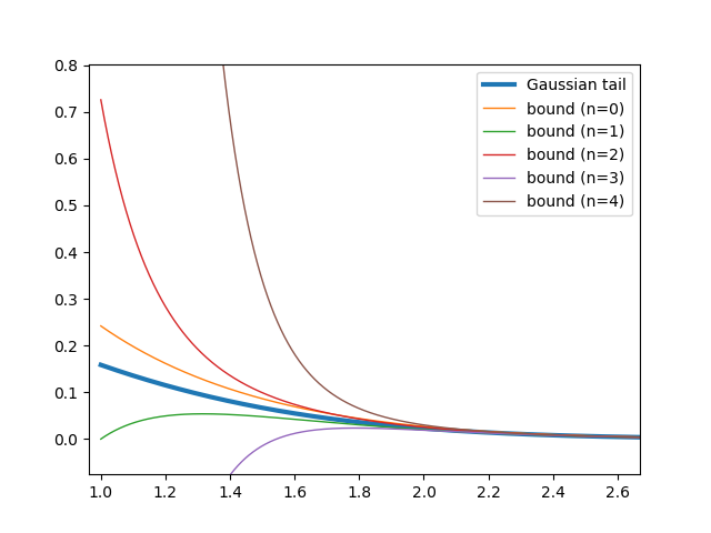
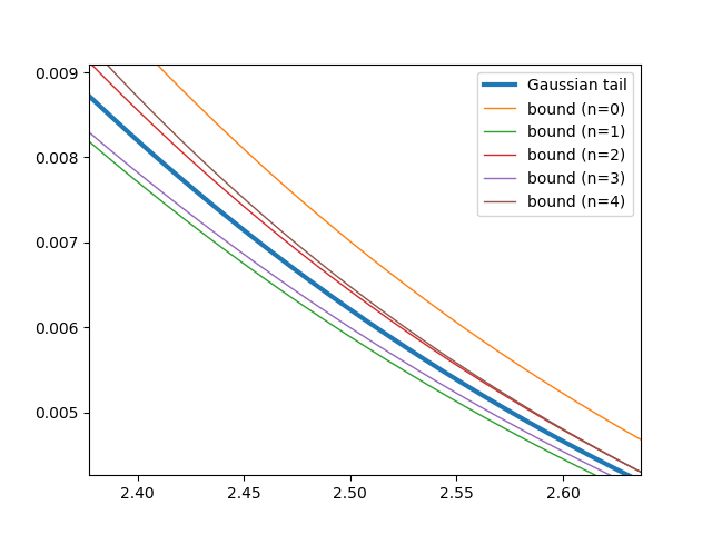
Plots of $x$ vs $1-\Phi(x)$.
Zoomed out view of the bounds for the first few n. Note the better tighter asymptotic bounds (larger n) aren't as tight for small x.

If we zoom in a bit on the tail, we can see the larger-n bounds becoming tighter:

Hazard Rates
The hazard rate of a distribution at $x$ is the conditional probability of $x$ given that the variable is at least $x$. If the random variable denotes the time of an event, then the hazard rate at $x$ is the probability that the event occurs at time $x$, given it has not occurred before $x$.
In particular, the above calculations give immediate and tight bounds on the hazard rate of the standard normal distribution, $h(x) = \frac{\phi(x)}{1-\Phi(x)}$. We get, for instance,
\[ \frac{1}{x} - \frac{1}{x^3} + \frac{3}{x^5} - \frac{15}{x^7} \leq \frac{1}{h(x)} \leq \frac{1}{x} - \frac{1}{x^3} + \frac{3}{x^5} . \]Perhaps surprisingly, the need for such tight bounds came up in a recent project of mine on bandit learning with Gaussian noise, when analyzing the variance of a Gaussian conditioned on exceeding a certain value. The more common $\frac{1}{x}\phi(x)$ upper bound turned out not to be tight enough. However, for most uses, even the subgaussian bound presented first is probably tight enough.

