Adversarial Binary Search (or, how to fleece Ballmer)

Posted: 2024-09-06.

This post describes how to solve an adversarial binary search game, inspired by an interview question of Steve Ballmer's.

Intro

A recent popular post discusses a Steve Ballmer interview question. I wanted to study the problem from a game-theoretic perpsective.

It's easy to define. Ballmer secretly picks an integer X between 1 and 100. The player, call her the Guesser, picks a number and learns whether it is correct, too high, or too low. The guesser continues until they get it right. Let's simplify by saying that Ballmer's utility is the number of steps, while the guesser's utility is the negative of this, making it a zero-sum game. (In the original formulation, the utilities were shifted by 6, i.e. if X is guessed in 4 steps, Ballmer pays Guesser 6 - 4 = 2 dollars.)

The main question: what is the value of this game? That is, what is the optimal expected number of guesses needed? In particular, we want to know if it is more or less than 6, i.e. if Ballmer makes or loses money.

This question is already not trivial if the upper bound is N=3 instead of N=100. The figure shows Ballmer's optimal strategy -- a probability distribution over which number X to pick -- and Guesser's optimal strategy for her first guess, also as a distribution.

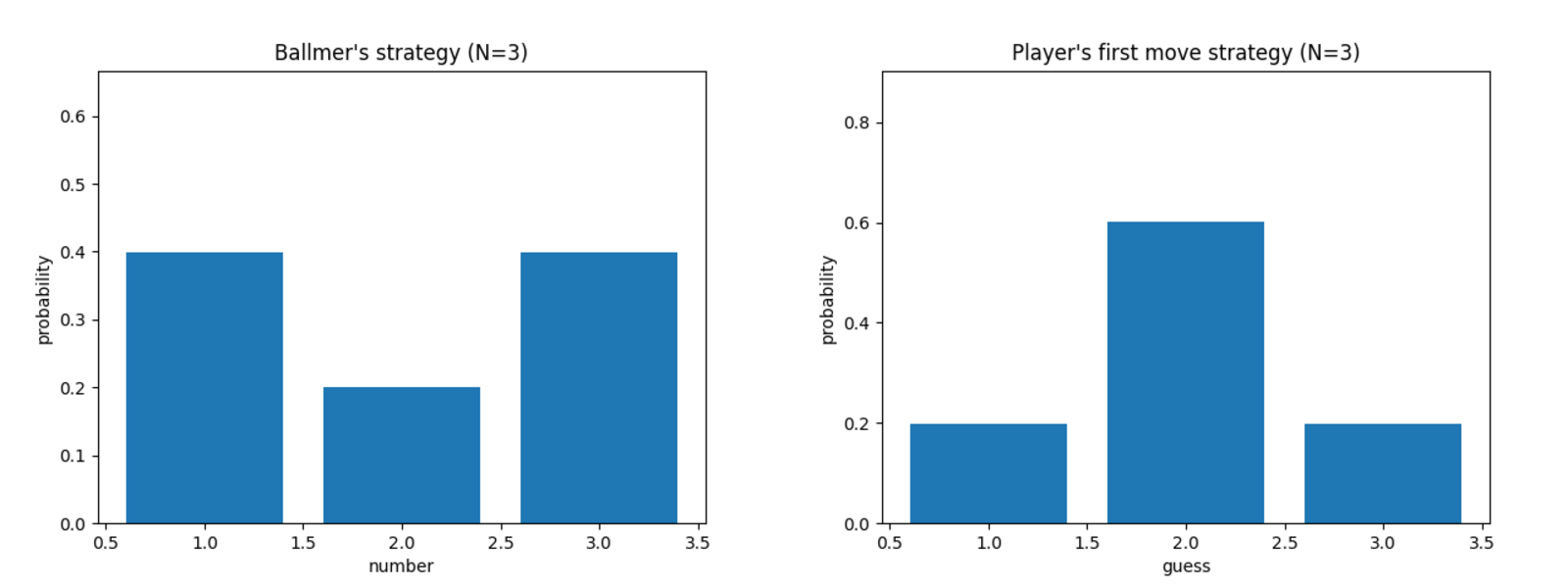
Ballmer draws X from the distribution Q = (0.4,0.2,0.4). The player's initial guess is drawn from (0.2,0.6,0.2). If the player initially guesses 2, their next guess (if any) is determined. If the player initially guesses 1, their next guess (if any) is 3, then 2. The case of 3 is symmetric.

One can check in this case that, no matter what X Ballmer picks, the expected number of steps is 1.8. (E.g. if X=1, there is a 0.2 probability of guessing it in one step, and a 0.8 probability of guessing in two steps; if X=2, there is a 0.6 probability of guessing in one step and a 0.4 probability of guessing in three steps.) Similarly, one can check that the player cannot do better than 1.8 against this strategy of Ballmer, so the value of the game for N=3 is 1.8.

As we increase N, it sort-of seems that a pattern emerges:

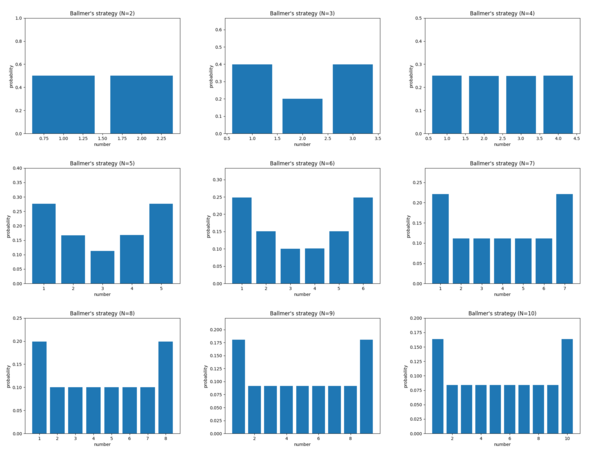
Above: Ballmer's strategies for N=2,...,10.
Below: Guesser's distribution of the first guess for N=2,...,10.

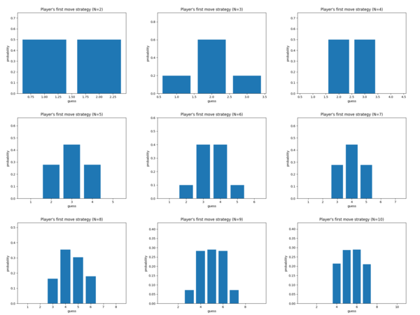
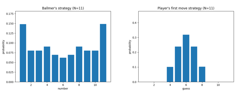
Does the pattern continue exactly this way? Not exactly! Here's N=11:

I don't see how to get a closed-form solution, so this post will talk about how I (approximately) numerically solved the game, including for N=100. Here's how we'll go about it:

• First steps
• Solving the game
• Some nitty gritty
• Evaluating the solution
• Guesser's mixed strategy
• Code

First steps

Let's start from the beginning. By using a standard binary search, Guesser can guarantee to end in 1 + floor(log2(100)) = 7 steps in the worst case. And if Ballmer cheats, i.e. doesn't commit to a number in advance, he can force the value to be 7 by always picking the side (above or below) with more remaining options.[1] Actually, for any deterministic guessing strategy, Ballmer can always commit in advance to some X that takes 7 or more steps to guess. So if Guesser wants to do better than 7, she has to use a randomized strategy.

How much better could she hope to do, on average? Well, we can analyze one simple strategy for Ballmer: pick the number uniformly at random. In this case, a best response for Guesser is to do a standard binary search. There is 1 option that is guessed on the first try; 2 options that are guessed on the second try; 4 on the third; 8 on the fourth; 16 on the fifth; 32 on the sixth; and the remaining 37 options are guessed in seven tries.[2] Each option occurs with probability 1/100, so this averages to (1*1 + 2*2 + 3*4 + 5*16 + 6*32 + 7*37)/100 = 5.8 guesses overall. So Ballmer has a mixed strategy (this means a randomized strategy) that guarantees the expected number of guesses is at least 5.8.

Ok: we know the value of the game is between 5.8 and 7. You might suggest that it's closer to 5.8, because it's hard to see how Ballmer does much better than picking totally at random. But on the other hand, we know that Guesser will have to randomize, or else Ballmer can force the value all the way to 7. Maybe this randomization hurts the average case performance of the binary search, so maybe the value is above 6 after all.

Solving the game

We can solve a 2-player zero-sum game using the online no-regret learning algorithm Multiplicative Weights. You can learn about the details in e.g. my lecture notes, but the general idea is:

1. Start with Player 1 playing uniformly at random.
2. Compute a best-response by Player 2.
3. Use the outcome of the game to update Player 1's strategy a little bit.
4. Repeat.

It's a theorem that, if we use Multiplicative Weights to update the distribution that Player 1 uses, then the time-average of strategies for both players form an approximate Nash equilibrium. The time average just means that we average the strategies used over all the time steps. In T rounds, we obtain an estimate of the value of the game that is accurate to within, at worst, sqrt(2 ln(K) / T), where K is the number of actions available to Player 1.

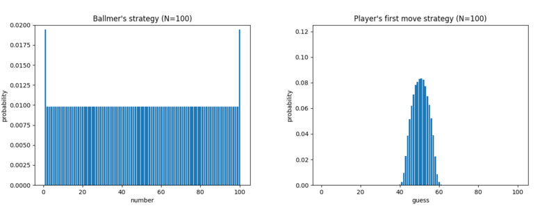
In our case, we'll take Player 1 to be Ballmer, who has 100 actions or "pure strategies" to choose from. We don't take Player 1 to be Guesser because she has way more pure strategies -- more on that later. By running Multiplicative Weights overnight on my desktop, I obtained the following strategy for Ballmer, and the following strategy for Guesser's first guess on round 1.

This supports the conjecture from our small examples that Ballmer's optimal strategy converges to the probability distribution

How to prove it? I have no idea. And I find it pretty counterintuitive that, for instance, he doesn't want to put lower probability on e.g. N/2. I guess the reason is that when Guesser plays a bit randomly, it's quite likely that N/2 is at the far end of a range, making it hard to guess.

Anyway, I also obtained the following for the approximate value of the game:

• Lower bound: 5.80371
• Estimage: 5.8039
• Upper bound: 5.81087

Some nitty gritty

One really nice feature of the online learning framework discussed above is that we only need to maintain a randomized strategy for one of the players, in this case, Ballmer. We only need a probability distribution over 100 actions. For the other player, Guesser, in each round we only have to compute a *pure strategy* best response to a given Ballmer distribution. That is, we never need to compute a randomized or mixed strategy for Guesser. That's huge, since even a pure strategy for Guesser is already a pretty complex object. We can think of it as a 2D array S, where S[a,b] is which index to guess when we've narrowed the range of possible values down to [a,b] inclusive. I'll talk about Guesser's randomized strategies toward the end of the post.

But to implement the online learning framework and evaluate it, we still have to solve a few nontrivial problems:

1. Given a mixed strategy Q for Ballmer, compute a best response strategy S for Guesser.
2. Given Guesser's strategy S, compute for each index the number of guesses it takes when that index is the correct answer.

Ok, the second one isn't too hard: given a pure strategy S for the guesser, we know that the index x = S[1,N] --- that is, the guess made when the remaining possible range is [1,N] --- is guessed in one step. It then splits the remaining numbers into two ranges, [1,x-1] and [x+1,N]. The indices S[1,x-1] and S[x+1,N] are guessed in two steps, and we then get 4 ranges (at most). Repeat.

The first problem is solvable with dynamic programming, but it takes a little thought. The base cases are ranges of width one. That is, for any a in 1...N, we can set S[a,a] = a. That is, the optimal guess, when the answer is known to be between a and a, is a. Similarly, the expected number of additional guesses needed in this case is 1, so we can create an array E and set E[a,a] = 1 for all a.

The key observation is that we need to induct on the width of the ranges we are solving for. For example, the next step is to solve all ranges of width 2, such as [57,58]. There, we just look at which index Ballmer would pick with higher probability. It's optimal to guess that index first, out of these two possibilities.

For general ranges [a,b], we consider each index i in [a,b] as a candidate guess. Assuming we guess i, the expected total number of additional steps is calculated by summing over the three possibilities, each weighted by its conditional probability given that Ballmer is drawing from Q conditioned on the range [a,b].

• If the true answer is less than i, then the answer is 1 + E[a,i-1]. This follows because we guess i (this takes one guess), then recurse on range [a,i-1].
• If the true answer is i, then the answer is 1 because we guess i.
• If the true answer is greater than i, then the answer is 1 + E[i+1,b].

By picking the minimum number of expected steps over all choices of i in [a,b], we obtain the strategy S[a,b] and the expected number of steps E[a,b]. To turn this into a DP algorithm, we need to iterate over range sizes from small to large, so our code should look like:

for a in [1,N]:
  E[a,a] = 1 and S[a,a] = a  # base cases
for width in [1,N]:
  for a in [1,N-width]:
    b = a + width
    for i in [a,b]:
      calculate expected number of additional steps (see above)
    S[a,b] = optimal choice of i
    E[a,b] = expected additional steps

Evaluating the solution

We have a theorem that the time-average strategies we get out of Multiplicative Weights form an approximate equilibrium. Specifically, in my simulations, the value of the game that I obtain, 5.803919, is guaranteed to be within +- 0.096 of the value from those two strategies playing each other. This guarantee isn't very good. Luckily, we can also just empirically check how good these strategies are. First, we take Ballmer's mixed strategy Q and compute a best-response. This is a pure-strategy best response, so it's the same dynamic-programming problem we were solving above. We get that the best Guesser can do against my computed Ballmer strategy is 5.80371. Compare this to the perfomance of Guesser's strategy that our algorithm found, which is 5.803919. Guesser is very close to best-responding.

Next, we take Guesser's mixed strategy and compute a best response from Ballmer. This is not too hard, as for each X=1,...,100, we just calculate the expected number of steps it takes to guess X, and take the worst case. This is again a dynamic programming problem with a similar structure. The main question is what Guesser's "mixed strategy" means, which I'll discuss on its own next. We get that the best Ballmer can do against the player strategy I computed is 5.81087. This is a gap of about 0.07, meaning that Ballmer is not quite best-responding. I suspect the true answer is much closer to 5.804, i.e. the lower end of the range. I think the gap arises because player strategies are complicated objects and take a while to converge (more in a moment).

Regardless, the computed strategies prove that the value of the game is in the range [5.80371, 5.81087], with an estimate of 5.804.

Guesser's mixed strategy

One of the trickiest parts of this project for me was thinking through Guesser's strategy space. As I mentioned, a pure strategy can be represented as a 2D array S where S[a,b] is the guess we make when we know the range is narrowed down to [a,b]. Of course, this leaves a lot of entries in the array meaningless because they are cases where a > b. More concerning, we have many entries that seem meaningful, but are never actually reached by this strategy. For example, if the first guess is 50, then we will never narrow down to the range [40,60], because we will always know whether the answer is above or below 50. So the entry S[40,60] will be meaningless in the context of this strategy.

This becomes important when trying to represent mixed strategies, which mean "probability distributions over pure strategies". If we're not careful, for example, if we simply average the two matrices for two strategies, then we'll miss the above fact in an important way and get the wrong answer.

Thinking about it this way, it's not clear that there even exists an efficient representation of a distribution over pure strategies. We would like to represent it e.g. as a 3D array, where the vector S[a,b] is a probability distribution over where we randomly choose to guess next given that we know the answer is in [a,b]. (Again, there are many unused entries.) We could calculate it by averaging, over all pure strategies in our distribution that can reach state [a,b], the guesses that they make. But this representation is clearly quite different than a probability distribution over pure strategies, where we first pick an entire strategy from the distribution, then follow it completely. For example, let A be the pure strategy of a classic binary search, while B is the pure strategy "Guess 100, then 99, then 98, ..., then 1." Suppose X=1. If we play A with probability 0.5 and B with probability 0.5, then the number of steps is 7 with probability 0.5 and is 100 with probability 0.5. If we use the matrix representation from 0.5A and 0.5B, then the number of steps is highly likely to be a number between 8 and 99, because e.g. when we reach the range [1,25], which we will, we have a half chance of going on to [1,12] and a half chance of going on to [1,24].

Luckily, we can argue that two representations have the same expected number of steps to guess any given X, so the 3D representation suffices. We use induction on the width of a range [a,b]. Conditioned on reaching this range, the distribution over our next guess is the same under both representations, and (by induction) the expected number of additional steps conditioned on any given guess is also the same.

So we can obtain an approximate equilibrium strategy for Guesser, in the form of a 3D matrix, by simply averaging the best-response pure strategies produced at each time step of the online learning process. We just have to be careful to only average in the strategy for ranges that actually happen for this pure strategy (e.g. the [40,60] example above). The result is linked in the code below. Here are some representations of certain rows as the distribution over the next guess, given that you have narrowed to [a,b].

Initial guess:

After guessing 57 and learning "lower":

After then guessing 27 and learning "higher":

Code

Notes: